[논문리뷰] Differentiable Motion Manifold Primitives for Reactive Motion Generation under Kinodynamic Constraints

논문 정보

• Title: Differentiable Motion Manifold Primitives for Reactive Motion Generation under Kinodynamic Constraints
• Authors: Yonghyeon Lee
• Venue / Year: IEEE International Conference on Robotics and Automation (ICRA), 2026
• Links: Paper, PDF, Project

한 줄 요약

Motion Manifold Primitives에 추가 training step을 도입해, 생성된 trajectory의 kinodynamic constraint satisfaction을 높이는 framework.

문제 정의

기존 MMP 계열의 학습 기반 motion generation 방법은 주로 demonstration data에 의존한다.

Optimization, sampling, search 기반 방법은 시스템의 차원이 높고 문제가 복잡할수록 computation time이 커져, 실시간 motion generation에 한계가 생길 수 있다.

또한 논문에서 다루는 기존 MMP 방법들은 학습 과정에 kinodynamic constraints를 명시적으로 반영하지 않아, 생성된 trajectory가 constraints를 위반할 수 있다.

핵심 아이디어

이러한 한계를 해결하기 위해 저자는 기존 Motion Manifold Primitives(MMP)를 확장해 kinodynamic constraints를 고려하는 Differentiable Motion Manifold Primitives(DMMP) 프레임워크를 제안한다.

Method

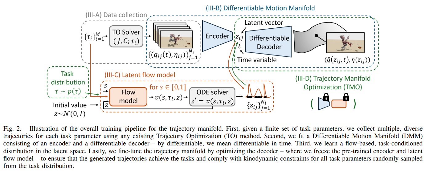
Training 전략은 다음 네 단계로 구성된다.

1. Data Collection via Trajectory Optimization : 여러 task parameter에 대해 trajectory optimization 문제를 풀어 다양한 trajectory를 수집한다.
2. Learning Differentiable Motion Manifold : 수집한 데이터로 시간에 대해 미분 가능한 trajectory를 생성하는 differentiable motion manifold를 학습한다.
3. Latent Flow Learning : 학습한 manifold의 latent space에서 task-conditioned latent flow model을 학습한다.
4. Trajectory Manifold Optimization : Encoder와 latent flow를 freeze하고 decoder만 fine-tuning해, 생성 trajectory의 task 수행과 kinodynamic constraint satisfaction을 개선한다.

Notation

기호	의미
$q\in Q\subset\mathbb{R}^{n}$	Configuration과 그 공간. $n$은 configuration dimension
$q(t)$	시간 $t$에서의 configuration을 나타내는 trajectory
$\tau\in\mathcal{T}$	Task parameter와 그 공간
$t\in[0,T]$, $T>0$	시간과 고정된 terminal time
$s=t/T$	Normalized time
$\eta$	specific한 motion 시점이 필요할때 쓰는 함수, i.e. Throwing task에서는 물체를 놓는 release time
$\dot q$, $\ddot q$, $\dddot q$	Configuration의 velocity, acceleration, jerk
$J(q(\cdot),\eta;\tau)$	Trajectory 전체와 $\eta$, task parameter에 의존하는 objective function
$C(q,\dot q,\ddot q,\dddot q)\in\mathbb{R}^{k}$	$k$개의 kinodynamic constraints를 표현하는 미분 가능한 함수. 각 성분이 0 이하여야 함
$\mathcal{T}s={\tau_i}{i=1}^{M}$	데이터 수집을 위해 선택한 $M$개 task parameter의 집합
$q_0$, $q_T$	Trajectory의 초기와 마지막 configuration
$B>1$	Basis function의 개수
$\Phi(s)\in\mathbb{R}^{1\times B}$	Gaussian basis function들을 모은 basis matrix
$w\in\mathbb{R}^{B\times n}$	Basis coefficient matrix

Data Collection via Trajectory Optimization

Objective Function

전체 task parameter space $\mathcal{T}$에서 유한한 집합 $\mathcal{T}_s$를 선택하고, 각 $\tau_i$에 대해 다음 문제를 푼다.

\[\begin{aligned} \min_{q(t),\eta}\quad & J(q(\cdot),\eta;\tau_i) \\ \text{s.t.}\quad & C(q,\dot q,\ddot q,\dddot q)\leq 0, \\ & \forall t\in[0,T]. \end{aligned}\]

Task parameter마다 초기값과 random seed를 바꾸어 문제를 여러 번 풀고, 다양한 trajectory를 수집한다.

Trajectory Parameterization

Trajectory $q(t)$는 다음과 같이 parameterize한다.

\[\begin{aligned} q(t) ={}& q_0+(q_T-q_0)(3-2s)s^2 +s^2(s-1)^2\Phi(s)w. \end{aligned}\]

여기서 normalized time은 다음과 같다.

\[s=\frac{t}{T}\in[0,1]\]

Basis matrix는 $B$개의 Gaussian basis function으로 구성한다.

\[\Phi(s) =\begin{bmatrix}\phi_1(s)&\cdots&\phi_B(s)\end{bmatrix} \in\mathbb{R}^{1\times B}\] \[\phi_i(s) =\exp\!\left[ -B^2\left(s-\frac{i-1}{B-1}\right)^2 \right], \qquad i=1,\ldots,B.\]

Learning Differentiable Motion Manifold

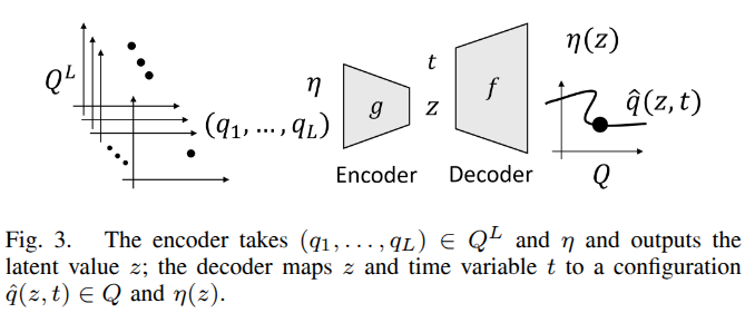
그림의 encoder $g$는 $L$개 시점에서 sample한 trajectory $(q_1,\ldots,q_L)$와 추가 변수 $\eta$를 입력받아 latent variable $z\in Z=\mathbb{R}^{m}$으로 embedding한다. 여기서 $m$은 latent dimension이다. Decoder $f$는 $z$와 시간 $t$를 입력받아 configuration $\hat q(z,t)$와 $\eta(z)$를 출력한다.

논문에서 비교하는 discrete-time MMP와 DMMP의 trajectory 출력 방식은 다음과 같다.

구분	Discrete-time MMP	DMMP
Decoder 입력	$z$	$(z,t)$
Trajectory 출력	고정된 시점의 configuration들을 모은 $(\hat q_1,\ldots,\hat q_L)$	입력한 시간 $t$에서의 configuration $\hat q(z,t)$

DMMP는 시간 $t$를 explicit input으로 받고, $\hat q(z,t)$가 $t$에 대해 미분 가능하도록 decoder를 구성한다.

Reconstruction Loss

이 단계에서는 encoder parameter $\alpha$와 decoder parameter $\beta$를 다음 reconstruction loss로 함께 학습한다. 두 오차 항을 각 task의 trajectory에 대해 평균하고, 다시 task 간 평균을 취한다.

\[\begin{aligned} \mathcal{L}_{\mathrm{recon}}(\alpha,\beta) \mathrel{:=}& \frac{1}{M}\sum_{i=1}^{M} \frac{1}{N_i}\sum_{j=1}^{N_i} \Bigl[ \left\|\hat q_\beta(z_{ij},t)-q_{ij}(t)\right\|_{c(t)}^2 + \left\|\eta_\beta(z_{ij})-\eta_{ij}\right\|^2 \Bigr]. \end{aligned}\]

$M$은 데이터 수집에 사용한 task parameter의 개수, $N_i$는 $\tau_i$에 대해 수집한 trajectory의 개수다. $z_{ij}$는 $\tau_i$의 $j$번째 trajectory와 $\eta_{ij}$를 encoder $g_\alpha$로 encoding한 latent variable이다.

1. $\hat q_\beta(z_{ij},t)-q_{ij}(t)$는 시간 $t$에서 decoder가 출력한 configuration과 원래 trajectory data의 configuration 차이 즉, trajecotry error라고 할수 있다.
2. $\eta_\beta(z_{ij})-\eta_{ij}$는 motion을 지정하는 데 필요한 추가 변수 $\eta$의 reconstruction error다. Throwing task에서 $\eta$는 물체를 놓는 release time이므로, decoder가 예측한 release time과 데이터의 release time 사이의 차이를 의미한다.

Trajectory error에 사용하는 norm에는 시간 가중치 $c(t)$가 다음과 같이 포함된다.

\[\left\|\delta(t)\right\|_{c(t)}^2 \mathrel{:=} \int_0^T c(t)\,\delta(t)^{\mathsf{T}}\delta(t)\,dt\]

여기서 $\delta(t)$는 trajectory error이며, $c(t)>0$는 시간에 따른 가중치다. 전체 시간 구간의 제곱 오차를 적분하되, $c(t)$가 큰 시점의 오차를 더 크게 반영한다.

Decoder Architecture

Memory와 computation efficiency를 높이기 위해 decoder의 trajectory 출력에 다음 linear basis function 구조를 사용한다.

\[\hat q_\beta(z,t) =\sum_{b=1}^{N_b}\psi_\beta^b(z)\,\theta_\beta^b(t)\]

여기서 $N_b$는 basis function의 개수다. $\psi_\beta^b(z)\in\mathbb{R}$는 $z$에 따라 결정되는 scalar coefficient이며, $\theta_\beta^b(t)\in\mathbb{R}^{n}$는 시간에 따른 basis function이다. 두 함수는 각각 neural network로 표현한다.

$z$를 고정하고 시간 $t$에 대해 미분하면 $\psi_\beta^b(z)$는 상수이므로, $\theta_\beta^b(t)$만 미분하면 된다. 따라서 coefficient network를 시간 미분하는 계산이 필요하지 않다.

또한 학습 후 고정된 $z$의 trajectory만 추론할 때는 $\psi_\beta(z)$를 한 번 계산해 저장하고 재사용할 수 있다. 이 경우 coefficient network 전체 대신 계수 값만 유지할 수 있어 memory 사용을 줄인다. 시간 basis를 계산하는 network는 계속 사용한다.

latent space $Z=\mathbb{R}^{m}$이 충분히 낮은 차원이고, mapping $z\mapsto\hat q_\beta(z,\cdot)$가 injective immersion 조건을 만족한다는 전제하에 생성된 trajectory 집합을 $m$차원 differentiable manifold로 해석한다. (다른 논문 인용 참고)

시간에 대해 smooth한 neural network로 decoder를 구성하면 $\hat q_\beta(z,t)$는 $t$에 대해 differentiable하다. 앞서 제시한 manifold 조건 아래에서, 이 trajectory들의 manifold를 Differentiable Motion Manifold(DMM)이라고 부른다.

Latent Flow Learning

이 단계에서는 MMFP 논문의 latent flow learning 방법을 사용한다.

Task-conditioned density $p(z\mid\tau)$는 multimodal이고 복잡한 nonconvex 구조를 가질 수 있으므로, 이를 표현하기 위해 flow-based generative model을 사용한다.

Latent flow model의 parameter를 $\gamma$로 두면, 학습한 conditional distribution $p_\gamma(z\mid\tau)$에서 $z$를 sample할 수 있다. 이렇게 sample한 $z$를 differentiable decoder에 넣어 motion을 생성하는 framework를 Differentiable Motion Manifold Flow Primitives(DMMFP)라고 부른다.

Trajectory Manifold Optimization

DMMFP가 생성한 trajectory는 kinodynamic constraints를 위반할 수 있다. 이러한 constraint violations를 줄이기 위해 Trajectory Manifold Optimization(TMO)로 manifold를 fine-tuning한다.

이때 encoder $g_\alpha$, decoder $f_\beta$, latent flow $p_\gamma$ 중 $\alpha$와 $\gamma$는 freeze하고, decoder parameter $\beta$만 추가 학습한다. 모든 모듈을 함께 학습하면 latent sampling과 ODE solver를 통해 backpropagation해야 하므로, decoder만 업데이트해 computation cost를 줄인다.

Task Loss

마지막 TMO 단계에서는 다음 task loss로 task objective와 kinodynamic constraint violations를 함께 고려한다.

\[\begin{aligned} \mathcal{L}_{\mathrm{task}}(\beta) \mathrel{:=}\mathbb{E}_{t,\tau,z}\Bigl[& J(\hat q_\beta(z,\cdot),\eta_\beta(z);\tau) \\ &+W^{\mathsf{T}}\!\left( \operatorname{ReLU}(C(t,z,\beta))^2 \right) \Bigr]. \end{aligned}\]

첫 번째 항 $J$는 생성한 motion이 주어진 task를 성공적으로 수행하도록 유도한다. 두 번째 항은 kinodynamic constraints를 위반한 정도에 penalty를 부여한다.

$\beta$는 decoder parameter이며, $W\in\mathbb{R}^{k}$는 각 constraint에 대한 양의 weight vector다. $C(t,z,\beta)$는 생성된 trajectory와 이를 미분하여, vel, acc, jerk를 고려한 constraint이다.

\[C(t,z,\beta) =C\!\left( \hat q_\beta, \frac{\partial\hat q_\beta}{\partial t}, \frac{\partial^2\hat q_\beta}{\partial t^2}, \frac{\partial^3\hat q_\beta}{\partial t^3} \right)\]

ReLU와 제곱은 $C(t,z,\beta)$의 각 성분에 적용하므로, 양수인 constraint violation의 제곱에 weight를 곱해 penalty를 계산한다.

$t$와 $\tau$는 각각 $[0,T]$와 $\mathcal{T}$에서 uniform하게 sample하고, $z$는 학습한 latent flow distribution $p_\gamma(z\mid\tau)$에서 sample한다.

Fine-Tuning Loss

앞서 정의한 reconstruction loss를 task loss와 함께 사용한다. 이 단계에서는 $\alpha$가 고정되어 있으므로 reconstruction loss를 $\mathcal{L}_{\mathrm{recon}}(\beta)$로 표기하고, 다음 loss를 최소화해 $\beta$를 학습한다.

\[\mathcal{L}(\beta) =w_{\mathrm{recon}}\mathcal{L}_{\mathrm{recon}}(\beta) +\mathcal{L}_{\mathrm{task}}(\beta)\]

여기서 $w_{\mathrm{recon}}>0$는 reconstruction loss의 weight다. 이 loss를 최소화하도록 decoder를 fine-tuning하는 과정을 Trajectory Manifold Optimization(TMO)라고 부른다.

TMO 이후에도 일부 trajectory가 constraints를 위반할 수 있으므로, fine-tuning 자체가 모든 생성 trajectory의 constraint satisfaction을 보장하는 것은 아니다.

Experiments

Dynamic Throwing with a 7-DoF Franka Panda Arm

7자유도 Franka Panda arm의 dynamic throwing task로 제안한 방법을 평가한다.

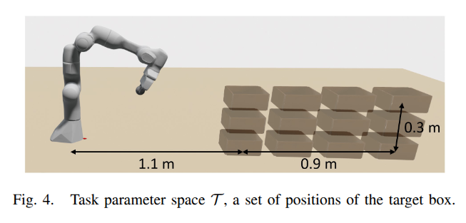
Task Parameter

Task parameter는 robot base를 기준으로 한 target box의 position이다.

\[\tau=(r\cos\theta,r\sin\theta,h)\in\mathbb{R}^{3}\]

여기서 $r$은 수평거리, $\theta$는 방위각, $h$는 높이다. 회전 대칭을 이용해 $\theta=0$인 task로 학습하고, $\theta\neq0$인 경우에는 첫 번째 joint를 해당 각도만큼 회전시켜 대응한다.

Objective

\[\begin{aligned} J(q(\cdot),\eta;\tau) ={}&J_{\mathrm{task}}(q(\cdot),\eta;\tau) \\ &+w_1\int_0^T\left\|\dddot q(t)\right\|^2\,dt. \end{aligned}\]

$J_{\mathrm{task}}$는 물체가 target box의 높이를 지날 때의 예상 위치와 target position 사이의 제곱 오차다. 두 번째 항은 전체 trajectory의 jerk 제곱을 적분한 penalty이며, $w_1$은 그 weight다.

Constraints

Joint position, velocity, acceleration, jerk, end-effector velocity, joint torque의 limits와 self-collision margins를 constraints로 둔다. Trajectory는 모든 시간에서 다음 조건을 만족해야 한다.

\[C(q,\dot q,\ddot q,\dddot q)\leq0, \qquad\forall t\in[0,T].\]

Data Collection

데이터 수집에 사용할 optimizer를 비교하기 위해 SLSQP, COBYLA, Adam의 optimization time과 convergence rate를 비교한다.

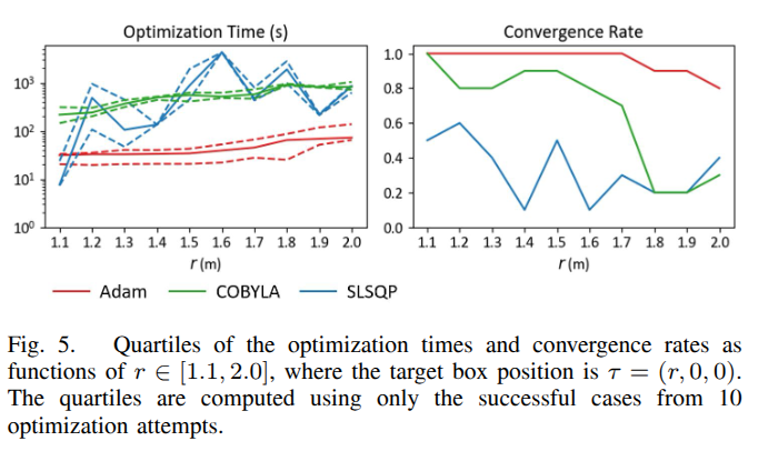
빨간색은 Adam, 초록색은 COBYLA, 파란색은 SLSQP다. $\tau=(r,0,0)$에서 거리를 바꾸며 각 조건마다 10번 시도했고, 왼쪽의 시간 사분위수는 성공한 시도만으로 계산했다. 오른쪽은 전체 시도 중 convergence한 비율이다.

비교 후 실제 trajectory 수집에는 Adam을 사용한다.

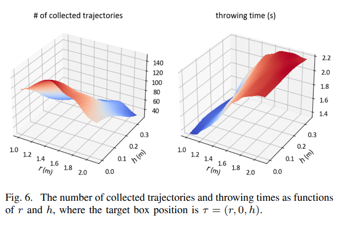
왼쪽은 $\tau=(r,0,h)$별 수집 trajectory 수, 오른쪽은 평균 release time $\eta$다. 각 그래프에서 빨간색은 큰 값, 파란색은 작은 값을 나타낸다. Target 거리가 멀어질수록 수집되는 trajectory가 줄고, release time이 늦어지는 경향을 보인다.

Planning Performance

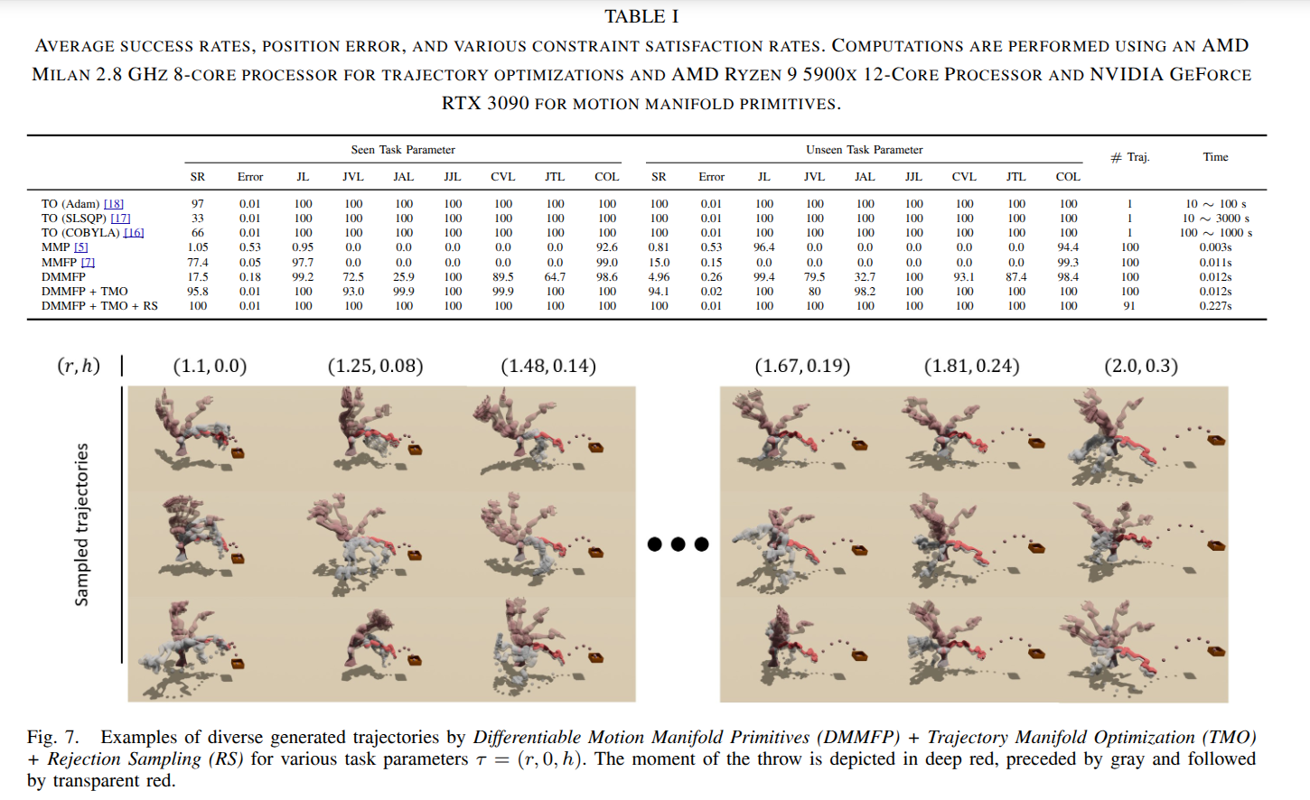
표는 seen, unseen task parameter에서의 성능을 비교한다. 아래 예시에서 회색은 throw 이전, 진한 빨간색은 release 순간, 연한 빨간색은 이후의 motion이다.

1. trajectory optimization이 manifold-based methods보다 훨씬 느리다. TO는 CPU에서 trajectory 하나를 생성하고, manifold 방식은 GPU를 활용해 100개를 병렬 생성하는 차이가 있다.
2. MMP, MMFP, DMMFP는 동일한 trajectory data에 fitting되지만, data fitting만으로는 constraints를 충분히 만족시키지 못한다. DMMFP는 constraint satisfaction에서 상대적으로 좋은데, 이를 temporal smoothness를 유도하는 inductive bias의 영향으로 해석한다. Task success 자체는 MMFP가 DMMFP보다 높다.
3. TMO를 적용하면 DMMFP의 task success가 seen에서 95.8%, unseen에서 94.1%로 높아진다. Residual constraint violation은 주로 Joint Velocity Limits(JVL)에 남으며, JVL satisfaction은 각각 93%, 80%다.
4. Rejection Sampling(RS)으로 조건을 만족하지 않는 sample을 제외하면, 이 실험에서 남긴 sample의 task success와 constraint satisfaction은 모두 100%가 된다.
5. RS에는 추가 constraint checking이 필요하므로 runtime이 증가한다. 표에서 DMMFP + TMO로 100개 sample을 생성하는 데 0.012 s가 걸리며, RS 검사까지 포함하면 0.227 s로 늘어난다.

Online Adaptation

동적으로 바뀌는 환경에 대응할 수 있는지 확인하기 위해, 시뮬레이션에서 throwing motion 도중 target box의 position을 변경한다. 모델은 바뀐 target에 맞춰 throwing trajectory를 다시 계획하고, transition trajectory로 현재 motion과 새 trajectory를 연결한다.

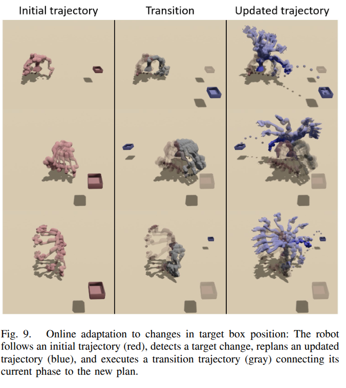
그림에서 빨간색은 기존 trajectory, 회색은 두 trajectory를 연결하는 transition, 파란색은 변경된 target에 대응하는 새 trajectory를 나타낸다.