CS185/285 (Spring 2026) - Deep Reinforcement Learning 1
00_Reinforcement Learning 개요
- Mathematical formalism for learning-based decision making
- Approach for learning decision making and control from experience
첫 번째는 mathematical formalism에 초점을 맞춘 좁은 의미의 RL이다. 두 번째는 경험을 통해 decision making과 control을 학습하는 접근을 포괄하는 넓은 의미의 RL이다.
넓은 의미에서는 구체적인 알고리즘이 Q-learning 등 기존 RL algorithms와 닮지 않았더라도, 시도와 그 결과에 대한 feedback을 바탕으로 이후의 의사결정을 개선하는 학습 패러다임을 포함한다.
시도 → 결과 관찰 → feedback에 따른 의사결정 수정
Standard (Supervised) Machine Learning vs. RL
standard supervised learning에서는 입력 $x$와 target $y$로 이루어진 dataset을 사용해, $x$로부터 $y$를 예측하는 model을 학습한다. RL과 비교할 때는 다음 두 가지를 구분할 수 있다.
i.i.d. Data
standard supervised learning 설정에서는 보통 data가 i.i.d.(independent and identically distributed)라고 가정한다. 즉, 데이터 쌍 $(x_i,y_i)$가 서로 independent하며 동일한 distribution에서 sample되었다고 가정한다.
RL에서는 이전 action이 이후 input에 영향을 줄 수 있다. 예를 들어 자율주행 차량의 카메라가 보는 화면은 이전에 선택한 action에 따라 달라진다. 따라서 상호작용으로 얻은 연속적인 experience에 i.i.d. 가정을 그대로 적용하기 어렵다.
Ground Truth
Supervised learning에서는 training data에 각 input의 target output $y$가 주어진다. Model은 예측값과 이 target을 비교하며 학습한다.
일반적인 RL 설정에서는 각 상황에서 선택해야 할 정답 action이 label로 주어지지 않는다. Agent는 action을 선택하고, 관측한 결과와 reward를 바탕으로 학습한다. Reward는 성공이나 실패를 나타내는 값일 수도 있고, 성능이나 비용을 반영하는 수치로 정의될 수도 있다.
01_Deep Reinforcement Learning의 필요성
Data-Driven AI와 RL
여기서는 data fitting과 goal optimization이라는 관점에서 장단점을 비교한다.
| 구분 | 장점 | 단점 |
|---|---|---|
| Data-Driven AI | Data로부터 real world의 패턴과 구조를 학습할 수 있다. | Data fitting만을 목표로 하면, 주어진 data보다 더 나은 행동을 찾는 optimization이 학습 목표에 직접 포함되지 않는다. |
| RL | Goal을 optimize하는 과정에서 미리 지정하지 않은 emergent behavior를 학습할 수 있다. | 한 task에서 학습한 policy를 다른 task로 transfer하거나 generalize하기 어려울 수 있다. |
The Bitter Lesson
교수님은 Richard Sutton이 2019년에 쓴 에세이 The Bitter Lesson을 읽어보기를 강력히 추천한다.
We have to learn the bitter lesson that building in how we think we think does not work in the long run.
The two methods that seem to scale arbitrarily … are learning and search.
Sutton은 우리가 생각하는 인간의 사고방식을 AI에 직접 설계해 넣는 접근에 장기적인 한계가 있다고 주장하며, 그 때문에 우리의 방법을 data를 통해 이해하는 learning뿐만 아니라 그 이해를 바탕으로 새로운 판단과 행동으로 연결하는 search가 필요하다고 말한다. 여기서 search는 goal을 달성하기위한 optimization과정이 포함된다.
재밌는 점은 사람들은 대부분 learning이 중요하다고 생각하고 learning에 집중하지만, search가 인간의 한계를 극복해주는 돌파구가 될수 있으므로, 이를 간과해서는 안된다.
Deep Learning과 RL의 결합
- Deep learning: 크고 복잡한 dataset에서 real world의 패턴과 유용한 representation을 학습한다.
- RL: Reward로 정의한 goal을 optimize해 더 나은 의사결정을 학습한다.
두 접근을 결합하는 목적은 real-world data에서 학습한 지식을 goal optimization에 활용해, simulator 밖의 현실 문제에도 적용하고 기존 data에 담긴 행동보다 더 나은 행동을 찾는 것이다.
02_Notation
Maximum Likelihood Estimation
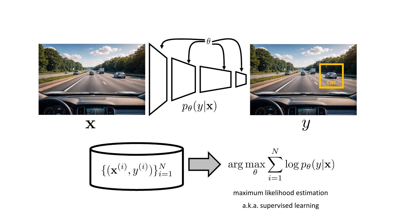
Supervised learning에서는 dataset의 입력 $\mathbf{x}$를 바탕으로 target $y$를 예측한다. 예를 들어 이미지 $\mathbf{x}$에서 물체의 종류와 위치에 해당하는 $y$를 예측하는 것이다.
모델을 conditional distribution $p_\theta(y\mid\mathbf{x})$로 표현하면, 다음 maximum likelihood estimation(MLE) 문제로 학습할 수 있다.
\[\theta^\star =\operatorname*{arg\,max}_{\theta} \sum_{i=1}^{N} \log p_\theta\!\left(y^{(i)}\mid\mathbf{x}^{(i)}\right)\]여기서 $N$은 training sample 수, $\theta$는 model parameter다. Dataset의 각 입력과 target 쌍에 대한 conditional log-likelihood의 합을 최대화한다.
Supervised Learning과 RL의 표기 비교
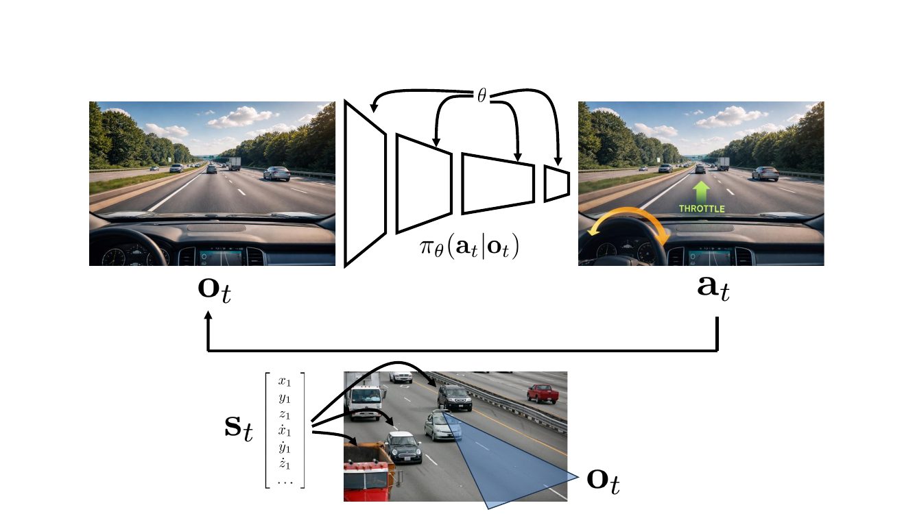
| Supervised Learning | Reinforcement Learning |
|---|---|
 |  |
03_State, Observation과 Markov Property
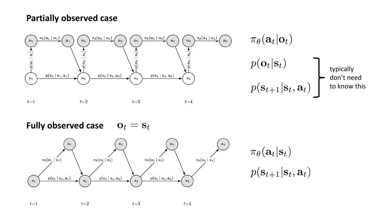
위쪽은 partially observed case, 아래쪽은 fully observed case다. 회색 원은 agent가 관측하는 변수, 흰색 원은 직접 관측하지 못하는 state이며, 화살표는 모델의 조건부 의존 관계를 나타낸다.
Partially Observed Case
Partially observed case에서는 현재 observation $o_t$만으로 측정 노이즈와 같은 노이즈 떄문에 state $s_t$를 정확하게 알수 없다. 또한 observation 자체는 일반적으로 Markov propoerty를 만족하지 않는다.
예를 즐다면 자율주행 차량의 오른쪽에 있던 자동차가 현재 카메라에서 보이지 않더라도, 잠시 관측 범위를 벗어났을 수 있다. 이때 과거 observation은 그 자동차가 여전히 주변에 있을 가능성을 추정하는 데 도움을 준다.
따라서 $\pi_\theta(a_t\mid o_t)$처럼 현재 observation만 사용하는 memoryless policy는 optimal policy를 표현하기에 부족할 수 있다.
Fully Observed Case
Fully observed case에서는 agent가 현재 state $s_t$를 직접 관측할 수 있으며, $o_t=s_t$로 둘 수 있다. 이때 state는 Markov property를 만족한다고 가정한다. 즉, 현재 state $s_t$와 action $a_t$가 주어졌을 때 다음 state $s_{t+1}$의 분포는 과거 state와 action에 추가로 의존하지 않는다.
\[\begin{aligned} &p(s_{t+1}\mid s_1,a_1,\ldots,s_t,a_t)\\ &\qquad=p(s_{t+1}\mid s_t,a_t) \end{aligned}\]즉, 다음 state를 예측하는 데 필요한 과거의 정보가 현재 state에 요약되어 있다는 뜻이다. 따라서 policy는
\[\pi_\theta(a_t\mid s_t)\]로 표현할 수 있다.
04_Behavior Cloning
Behavior cloning은 demonstration trajectory의 observation과 action 쌍을 supervised learning data로 사용해, expert의 행동을 모방하는 policy를 학습하는 방법이다.
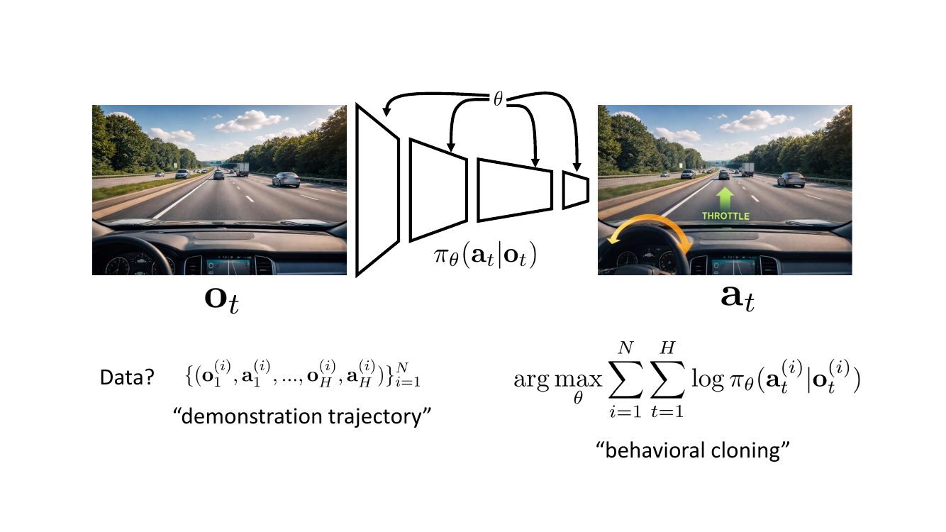
그림에서 주황색 화살표는 steering, 초록색 화살표는 throttle action이다. $N$개의 demonstration trajectory가 있고 각 trajectory의 길이를 $H$로 두면, 다음 objective를 최대화한다.
\[\theta^\star =\operatorname*{arg\,max}_{\theta} \sum_{i=1}^{N}\sum_{t=1}^{H} \log\pi_\theta\!\left(a_t^{(i)}\mid o_t^{(i)}\right)\]여기서 $o_t^{(i)}$, $a_t^{(i)}$는 $i$번째 demonstration의 시간 $t$에서 관측한 observation과 expert action이다.
Discrete Action과 Continuous Action
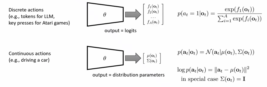
위쪽은 discrete action, 아래쪽은 continuous action을 Gaussian으로 모델링하는 경우다. 회색 화살표는 network가 각각 logits와 distribution parameters를 출력하는 흐름을 나타낸다.
Discrete Action
Discrete action이 $A$개라면 network는 $A$차원의 logit vector를 출력한다. 각 logit을 $f_k(o_t)$로 쓰면, softmax를 통해 action probability를 얻는다.
\[\pi_\theta(a_t=k\mid o_t) =\frac{\exp(f_k(o_t))}{\sum_{j=1}^{A}\exp(f_j(o_t))}\]Logit vector는 network의 output이며, loss는 이 확률과 demonstration의 expert action을 이용해 계산한다.
Continuous Action
Continuous action을 multivariate Gaussian으로 모델링하면, network는 mean $\mu_\theta(o_t)$와 covariance $\Sigma_\theta(o_t)$를 parameterize한다.
\[\pi_\theta(a_t\mid o_t) =\mathcal{N}\!\left(a_t\mid\mu_\theta(o_t),\Sigma_\theta(o_t)\right)\]Covariance를 $I$로 고정하면 negative log-likelihood는 다음과 같이 단순화된다.
\[-\log\pi_\theta(a_t\mid o_t) =\frac{1}{2}\left\|a_t-\mu_\theta(o_t)\right\|_2^2 +\mathrm{const}\]$\mathrm{const}$는 $\theta$에 무관한 항이다. 따라서 이 조건에서는 expert action과 예측한 mean 사이의 squared error를 최소화하는 학습이 된다. 그림 아래의 log-likelihood 등식은 부호와 계수가 맞지 않으므로, 정확한 negative log-likelihood는 위 식으로 정리한다.
05_Does Behavior Cloning Work?
Failure Case: Error Accumulation
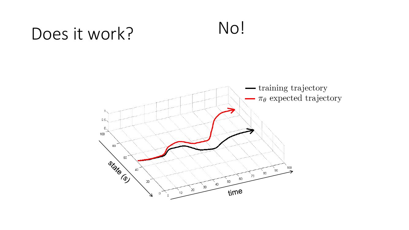
검은 선은 training trajectory, 빨간 선은 학습한 policy $\pi_\theta$의 예상 trajectory다. 처음에는 작은 action error라도, 그 행동이 이후에 방문하는 state를 바꾸면서 expert data에서 거의 보지 못한 상황으로 이어질 수 있다. 이 상황에서 다시 실수하면 error가 누적되어 trajectory가 더 크게 벗어날 수 있다.
이는 expert의 training data와 학습한 policy가 실제 rollout에서 만나는 data 사이의 distribution shift 문제다. behavior cloning이 항상 실패한다는 뜻은 아니지만, 벗어난 상황에서의 복귀 행동을 배우지 못하면 작은 예측 오차가 큰 실행 오차로 이어질 수 있다.
Work Example: NVIDIA
NVIDIA의 Bojarski et al. (2016)은 카메라 이미지에서 steering command를 직접 예측하는 CNN을 학습해 차량을 주행시켰다. 이때 실수로 경로를 벗어났을 때의 복귀 행동을 학습하도록 data augmentation을 사용했다.
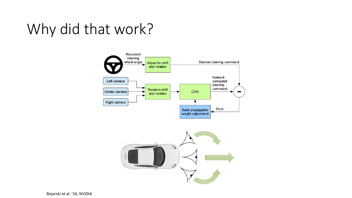
학습할 때는 center, left, right camera에서 얻은 이미지를 각각 training sample로 사용한다. Left와 right camera의 시점은 차량이 중심선에서 좌우로 벗어난 상황을 나타내는 데 활용한다. 같은 진행 방향에서 왼쪽으로 치우친 시점에는 오른쪽으로 복귀하는 steering 보정을, 오른쪽으로 치우친 시점에는 왼쪽으로 복귀하는 보정을 원래 label에 반영한다.
추가로 이미지에 random shift와 rotation을 적용하고, 바뀐 위치와 방향에서 원하는 경로로 돌아오도록 steering label도 함께 조정한다. 그림의 초록색 shift, rotation 블록들은 이 image와 label의 보정을 나타내며, 아래 초록색 화살표는 직진과 좌우 이탈에 대한 복귀 조향을 보여준다.
이렇게 학습한 뒤 실제 주행에서 steering을 예측할 때는 center camera 하나만 사용한다. 세 카메라와 augmentation은 중심선에서 벗어난 시점과 그에 맞는 복귀 행동을 training data에 포함시키는 역할을 한다.
Distributional Shift
앞에서 Behavior cloning이 이론적으로는 안되었는데 하나의 trick으로 되게 만든 예시를 보았다. 이렇게 behavior cloning을 막는 현상을 Distribution shift라고 한다.
이는 모델 $p_\theta(y\mid\mathbf{x})$를 학습할 때와 test할 때 입력 $\mathbf{x}$의 distribution이 달라지는 현상이다.
\[\begin{aligned} \text{Training:}\quad&\mathbf{x}\sim p_{\mathrm{train}}(\mathbf{x}) \\ \text{Test:}\quad&\mathbf{x}\sim p_{\mathrm{test}}(\mathbf{x}) \\ &p_{\mathrm{test}}(\mathbf{x})\neq p_{\mathrm{train}}(\mathbf{x}) \end{aligned}\]예를 들자면, 수학을 공부했는데 문학 시험을 보는 상황은 학습한 내용과 test에서 마주하는 내용이 다른 상황이라고 할수 있다. 이는 task 자체가 바뀌지 않더라도, 같은 task를 계속 진행하면서 익숙하지 않은 state를 만날때 발생한다.
Control에서는 action이 다음 state와 observation에 영향을 주므로, i.i.d조건이 깨지며 expert와 학습한 policy가 서로 다른 state distribution을 만들 수 있다. 따라서 외부 환경이 바뀌지 않아도 policy를 실행하는 과정에서 distribution shift가 생길 수 있다.
06_How bad it could be?
이론적으로 해당현상이 behavior cloning을 얼마나 나쁘게 만들 수 있는지를 이해한다. 이떄, 이론적 분석의 우리에게 주는 것이 어떤것인지 구분할 수 있어야한다.

즉, 이론이 줄수있는건 trade-off에 대한 직관이고 어떻게 나쁘게 되는지를 이해한다. 우리는 이론적 증명을 실용적으로 사용과 연결지어서는 안된다.
Setup
분석을 단순하게 하기 위해 fully observable setting, 즉 $o_t=s_t$인 경우를 생각한다. Data는 좋은 policy $\pi^\star$가 생성한다고 하자. 이 policy는 deterministic하다. state $s_t$에서 올바른 action은 $\pi^\star(s_t)$다.
cost function은 단순하게 error가 발생할때마다 1을 지불해야하는 함수로 정의한다.
\[c(s_t,a_t)= \begin{cases} 0 & \text{if } a_t=\pi^\star(s_t),\\ 1 & \text{otherwise}. \end{cases}\]정의한 cost function을 사용한 expected value는 다음과 같은데,
\[\begin{aligned} \mathbb{E}_{a_t\sim\pi_\theta(\cdot\mid s_t)}[c(s_t,a_t)] &=\sum_{a_t}\pi_\theta(a_t\mid s_t)c(s_t,a_t) \\ &=\sum_{a_t\neq\pi^\star(s_t)}\pi_\theta(a_t\mid s_t) \\ &=\pi_\theta\!\left(a_t\neq\pi^\star(s_t)\mid s_t\right). \end{aligned}\]이는 state $s_t$가 주어졌을 때 expert와 다른 action을 선택할 확률이다.
Trajectory 관점에서의 Expected Total Errors
한 state에서의 실수 확률뿐만 아니라, 학습한 policy가 실제 rollout에서 방문하는 state 분포를 고려해 전체 trajectory에서 얼마나 error가 발생하는지를 평가해야 한다.
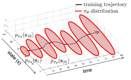
검은 선은 training trajectory, 붉은 타원은 각 시점에서 policy $\pi_\theta$가 유도하는 state distribution $p_{\pi_\theta}(s_t)$를 나타낸다.
Horizon이 $H$인 한 trajectory의 total cost는 $\sum_{t=1}^{H}c(s_t,a_t)$다.
\[\begin{aligned} &\mathbb{E}_{\pi_\theta}\!\left[\sum_{t=1}^{H}c(s_t,a_t)\right] =\sum_{t=1}^{H} \mathbb{E}_{\substack{ s_t\sim p_{\pi_\theta}(s_t),\; a_t\sim\pi_\theta(\cdot\mid s_t) }} \left[c(s_t,a_t)\right]. \end{aligned}\]앞서 정의한 0-1 cost에서는 이 값이 전체 trajectory에서 expert와 다른 action을 선택하는 횟수의 expectation이다.
$p_{\pi_\theta}(s_t)$는 $\pi_\theta$를 실행했을 때 시간 $t$에서의 state distribution이다. 초기 state distribution과 environment dynamics, 그리고 이전 시점들에서 policy가 선택한 action들의 영향을 반영한다.
Worst-Case Situation
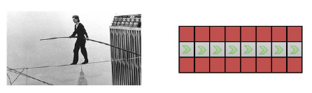
왼쪽 그림의 줄타기나, 오른쪽 그림의 단일 경로만 존재하는 통로를 지나는 문제를 생각해보자.
해당 경우에서 expert trajectory상의 state 집합을 $\mathcal{D}_{\mathrm{train}}$으로 둔다.
\[\pi_\theta\!\left(a\neq\pi^\star(s)\mid s\right)\leq\epsilon,\qquad\forall s\in\mathcal{D}_{\mathrm{train}}.\]해당 state에서의 one-step action error 확률은 $\epsilon$ 보다 작다.
첫 step에서 error가 발생하면 앞으로 모든 step은 $H$는 error가 된다. error가 아니면 남은 $H-1$ step에 같은 분석을 적용한다. 이를 반복하면 expected total cost의 bound는 다음과 같다.
\[\begin{aligned} &\sum_{t=1}^{H} \mathbb{E}_{\substack{ s_t\sim p_{\pi_\theta}(s_t), a_t\sim\pi_\theta(\cdot\mid s_t) }}[c(s_t,a_t)] \\ &\quad\leq\epsilon H+(1-\epsilon) \bigl(\epsilon(H-1)+(1-\epsilon)(\cdots)\bigr) \\ &\quad\leq\frac{\epsilon H(H+1)}{2} =O(\epsilon H^2). \end{aligned}\]이는 one-step error가 작더라도 worst-case에서는 그 영향이 이후 step으로 이어지면서 expected total errors가 크게 누적될 수 있음을 보여준다.
More General Analysis
앞에서는 각 expert state에서 action error 확률이 $\epsilon$ 이하라고 가정했다. 이번에는 각 시점 $t$의 expert state distribution에서 평균한 error 확률이 $\epsilon$ 이하라고 가정한다.
\[\mathbb{E}_{s_t\sim p_{\mathrm{train}}(s_t)} \left[\pi_\theta\!\left(a_t\neq\pi^\star(s_t)\mid s_t\right)\right] \leq\epsilon\]training distribution에서 state 하나를 sample하면, policy가 error를 낼 가능성은 크지 않다.
policy가 유도하는 state distribution $p_{\pi_\theta}(s_t)$를 시각 t까지 error를 낸적이 있는가에 따라 두분으로 나눈다.
\[\begin{aligned} p_{\pi_\theta}(s_t) ={}&(1-\epsilon)^t p_{\mathrm{train}}(s_t) +\bigl(1-(1-\epsilon)^t\bigr)p_{\mathrm{mistake}}(s_t) \end{aligned}\]TV divergence활용한 비교
TV divergence를 활용해 $p_{\mathrm{train}}$과 $p_{\pi_\theta}$를 비교해보자.
-
TV divergence를 사용하여, 식을 전개한다.
\[\begin{aligned} &D_{\mathrm{TV}}(p_{\mathrm{train}},p_{\pi_\theta})=\frac{1}{2}\sum_{s_t}\Bigl| p_{\mathrm{train}}(s_t)-(1-\epsilon)^t p_{\mathrm{train}}(s_t)-(1-(1-\epsilon)^t)p_{\mathrm{mistake}}(s_t) \Bigr| \end{aligned}\] -
$1-(1-\epsilon)^t\geq0$이므로 절댓값 밖으로 꺼낼 수 있다.
\[\begin{aligned} D_{\mathrm{TV}}(p_{\mathrm{train}},p_{\pi_\theta}) &=(1-(1-\epsilon)^t)\frac{1}{2}\sum_{s_t} \left|p_{\mathrm{train}}(s_t)-p_{\mathrm{mistake}}(s_t)\right| \\ &=(1-(1-\epsilon)^t)D_{\mathrm{TV}}(p_{\mathrm{train}},p_{\mathrm{mistake}}) \end{aligned}\] -
$D_{\mathrm{TV}}\leq1$을 사용한다.
\[D_{\mathrm{TV}}(p_{\mathrm{train}},p_{\pi_\theta}) \leq1-(1-\epsilon)^t\] -
$\epsilon\in[0,1]$이고 $t$가 양의 정수이면 Bernoulli inequality에 의해 $(1-\epsilon)^t\geq1-\epsilon t$다. 따라서 다음을 얻는다.
\[D_{\mathrm{TV}}(p_{\mathrm{train}},p_{\pi_\theta}) \leq1-(1-\epsilon)^t \leq\epsilon t\]
즉, t가 클수록 멀어진다. 이것이 error accumulation이 수학적으로 표현한것이다.
Expected Total Number of Errors
이제 실제로 관심 있는 expected total number of errors를 다시 생각한다.
Expected total cost를 $J(\pi_\theta)$로 쓰면, state에 대한 expectation을 전개해 다음과 같이 표현할 수 있다.
\[\begin{aligned} J(\pi_\theta) &=\sum_{t=1}^{H} \mathbb{E}_{\substack{ s_t\sim p_{\pi_\theta}(s_t), a_t\sim\pi_\theta(\cdot\mid s_t) }}[c(s_t,a_t)] =\sum_{t=1}^{H}\sum_{s_t} p_{\pi_\theta}(s_t)\mathbb{E}_{a_t\sim\pi_\theta(\cdot\mid s_t)}[c(s_t,a_t)]. \end{aligned}\]$p_{\mathrm{train}}(s_t)$를 더하고 빼서, training distribution에서의 error와 distribution shift에 따른 항으로 나눈다.
\[\begin{aligned} J(\pi_\theta) ={}&\sum_{t=1}^{H}\Bigl[ \sum_{s_t}p_{\mathrm{train}}(s_t)\mathbb{E}_{a_t\sim\pi_\theta(\cdot\mid s_t)}[c(s_t,a_t)]+\sum_{s_t} \bigl(p_{\pi_\theta}(s_t)-p_{\mathrm{train}}(s_t)\bigr) \mathbb{E}_{a_t\sim\pi_\theta(\cdot\mid s_t)}[c(s_t,a_t)] \Bigr] \\ \leq{}&\sum_{t=1}^{H}\Bigl[ \sum_{s_t}p_{\mathrm{train}}(s_t)\mathbb{E}_{a_t\sim\pi_\theta(\cdot\mid s_t)}[c(s_t,a_t)]+\sum_{s_t} \left|p_{\pi_\theta}(s_t)-p_{\mathrm{train}}(s_t)\right| \mathbb{E}_{a_t\sim\pi_\theta(\cdot\mid s_t)}[c(s_t,a_t)] \Bigr]. \end{aligned}\]마지막 단계는 $\mathbb{E}{a_t\sim\pi\theta(\cdot\mid s_t)}[c(s_t,a_t)]\geq0$을 사용한 upper bound다.
첫 번째 항은 앞서 가정한 training distribution에서의 평균 action error이므로 $\epsilon$ 이하이다.
\[\sum_{s_t}p_{\mathrm{train}}(s_t)\mathbb{E}_{a_t\sim\pi_\theta(\cdot\mid s_t)}[c(s_t,a_t)] =\mathbb{E}_{s_t\sim p_{\mathrm{train}}(s_t)}[\mathbb{E}_{a_t\sim\pi_\theta(\cdot\mid s_t)}[c(s_t,a_t)]] \leq\epsilon\]두 번째 항은 $\mathbb{E}{a_t\sim\pi\theta(\cdot\mid s_t)}[c(s_t,a_t)]\leq1$과 TV bound를 사용한다.
\[\begin{aligned} \sum_{s_t} \left|p_{\pi_\theta}(s_t)-p_{\mathrm{train}}(s_t)\right| \mathbb{E}_{a_t\sim\pi_\theta(\cdot\mid s_t)}[c(s_t,a_t)]&\leq\sum_{s_t} \left|p_{\pi_\theta}(s_t)-p_{\mathrm{train}}(s_t)\right| \\ &=2D_{\mathrm{TV}}(p_{\pi_\theta},p_{\mathrm{train}}) \leq2\epsilon t. \end{aligned}\]따라서 다음 bound를 얻는다.
\[J(\pi_\theta) \leq\sum_{t=1}^{H}(\epsilon+2\epsilon t) =O(\epsilon H^2)\]Test에서도 training과 같은 distribution을 만나고 각 prediction의 평균 error가 $\epsilon$ 이하인 supervised learning이라면, $H$개 prediction의 expected total errors는 $\epsilon H$, 즉 $O(\epsilon H)$로 bound된다. 반면 expert data에 fitting한 behavior cloning은 자신의 rollout에서 distribution shift를 만들 수 있어, worst-case bound가 $O(\epsilon H^2)$가 된다.
Why Is This Rather Pessimistic?
Worst-case 분석이 가정한 상황이 현실에서 항상 나타나는 것은 아닌데, 실제 시스템에서는 작은 오차가 생겨도 다시 원하는 경로로 돌아올 수 있는 경우가 있으며, 이를 위한 controller나 recovery 동작을 설계할 수도 있다.
다만 회복이 가능하다는 것과 policy가 회복 방법을 학습했다는 것은 다르다. 정상적인 expert trajectory만 학습한 behavior cloning은 경로를 벗어난 state에서 어떤 action을 해야 하는지 충분히 배우지 못할 수 있다. 일반적인 behavior cloning 학습 절차에는 learner가 새로 방문한 state의 expert label을 자동으로 추가하는 과정이 없다. 앞의 NVIDIA 사례처럼 recovery data를 별도로 포함하면 behavior cloning으로도 복귀 행동을 학습할 수 있다.
07_DAgger: Dataset Aggregation
DAgger는 behavior cloning이 새로 방문한 state의 정보가 없는 것을 고려하여 추가적인 dataset을 aggregation하는 방법이다
구체적인 방법으로는 학습한 policy가 방문하는 observation에 expert action label을 붙이고, 이를 기존 dataset에 추가하며 policy를 반복 학습한다.
DAgger Algorithm
초기 expert dataset을 다음과 같이 둔다. $N$은 observation-action 쌍의 개수이며, $a_i^\star$는 expert가 제공한 action label이다.
\[\mathcal{D}=\{(o_i,a_i^\star)\}_{i=1}^{N}\]- 초기 데이터셋으로 학습을 진행한다.
- 학습된 데이터로 작업을 진행한다.
- 진행된 작업중 일부를 사람이 적절한 action에 label해준다.
- label한 데이터와 기존 데이터셋을 합친다.
1~4번과정을 계속 반복하는 방식이 DAgger Algorithm이다.
Human Intervention을 사용하는 Variant
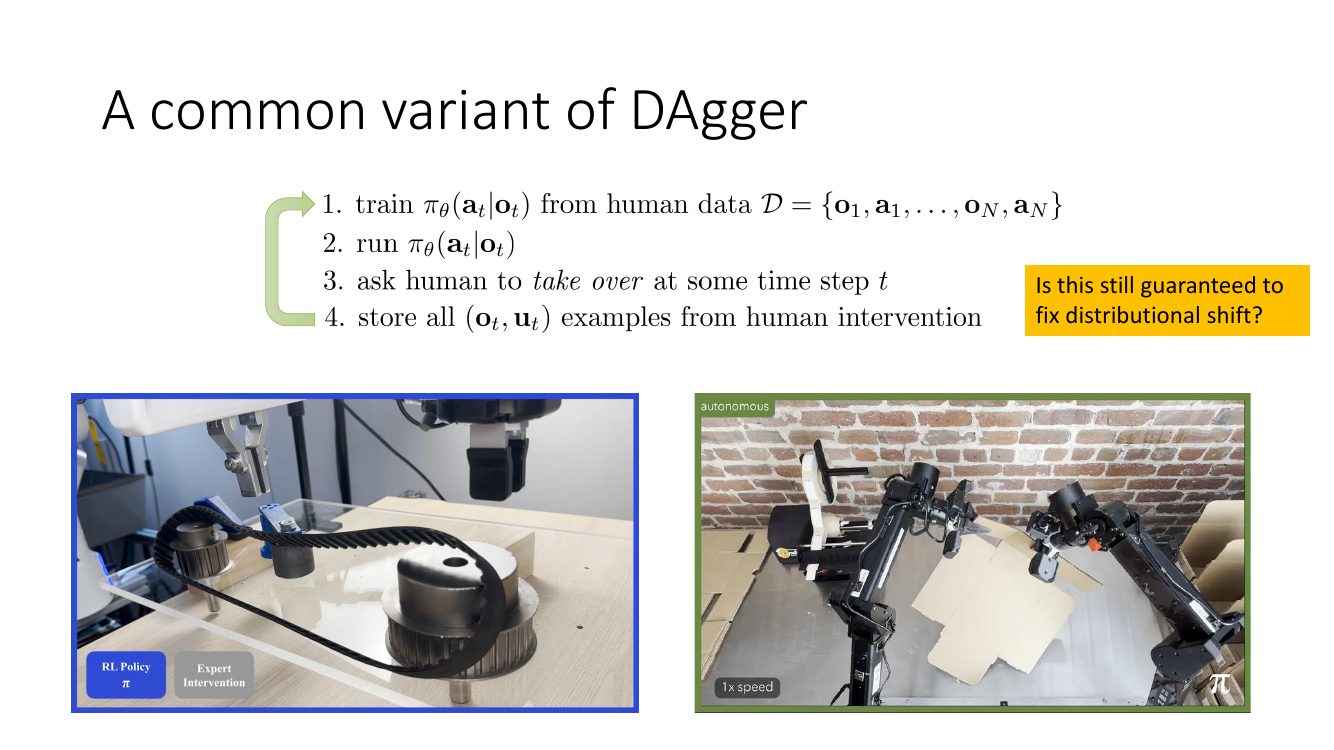
DAgger Algorithm은 일부 state를 사람들이 가져와서 적절한 action으로 labelling해줘야하는데 이를 개선한 방법이 등장한다.
기존과 달리 이 방식에서는 특정 $t$ step에서 사람이 직접 개입하여 획득한 정보를 dataset에 추가하여 학습하게 된다.
새 data가 사람이 선택한 개입 구간에서 수집되므로, 개입 시점에 대한 주관적인 판단에 따라 수집 분포가 편향될 수 있으며, 개입하지 않은 상황에서는 expert label을 충분히 얻지 못할 수도 있는 단점이 존재한다.
Intervention data를 누적해 재학습하면 recovery 행동과 성능을 개선시킬 수 있다.