[PythonRobotics 분석] LQR_steer_control 분석(Infitie Horzion)
main 코드
def main():
    print("LQR steering control tracking start!!")
    ax = [0.0, 6.0, 12.5, 10.0, 7.5, 3.0, -1.0]
    ay = [0.0, -3.0, -5.0, 6.5, 3.0, 5.0, -2.0]
    goal = [ax[-1], ay[-1]]

    cx, cy, cyaw, ck, s = cubic_spline_planner.calc_spline_course(
        ax, ay, ds=0.1)
    target_speed = 10.0 / 3.6  # simulation parameter km/h -> m/s

    sp = calc_speed_profile(cx, cy, cyaw, target_speed)

    t, x, y, yaw, v = closed_loop_prediction(cx, cy, cyaw, ck, sp, goal)
여기서 cubic_spline_planner는 점을 ds길이에 맞게, interpolate한 점들을 연산해준다.
그래서 나오는 cx, cy, cyaw, ck, s는 생겨난 경로의 특정 지점들의 집합이라고 생각하면된다.
(k : 곡률)
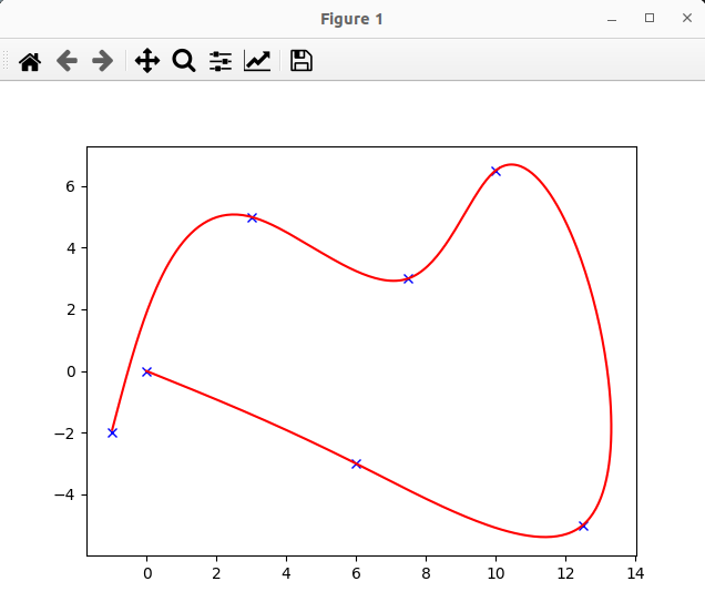
interpolate된 경로
Speed Profile생성
def calc_speed_profile(cx, cy, cyaw, target_speed):
    speed_profile = [target_speed] * len(cx)

    direction = 1.0

    # Set stop point
    for i in range(len(cx) - 1):
        dyaw = abs(cyaw[i + 1] - cyaw[i])
        switch = math.pi / 4.0 <= dyaw < math.pi / 2.0

        if switch:
            direction *= -1

        if direction != 1.0:
            speed_profile[i] = - target_speed
        else:
            speed_profile[i] = target_speed

        if switch:
            speed_profile[i] = 0.0

    speed_profile[-1] = 0.0

    return speed_profile
$\Delta \theta$가 45도 이상 90도 미만일 경우, 차량의 방향을 바꾼다.
메인 loop
def closed_loop_prediction(cx, cy, cyaw, ck, speed_profile, goal):
    T = 500.0  # max simulation time
    goal_dis = 0.3
    stop_speed = 0.05

    state = State(x=-0.0, y=-0.0, yaw=0.0, v=0.0)

    time = 0.0
    x = [state.x]
    y = [state.y]
    yaw = [state.yaw]
    v = [state.v]
    t = [0.0]

    e, e_th = 0.0, 0.0

    while T >= time:
        dl, target_ind, e, e_th = lqr_steering_control(
            state, cx, cy, cyaw, ck, e, e_th)

        ai = pid_control(speed_profile[target_ind], state.v)
        state = update(state, ai, dl)

        if abs(state.v) <= stop_speed:
            target_ind += 1

        time = time + dt

        # check goal
        dx = state.x - goal[0]
        dy = state.y - goal[1]
        if math.hypot(dx, dy) <= goal_dis:
            print("Goal")
            break

        x.append(state.x)
        y.append(state.y)
        yaw.append(state.yaw)
        v.append(state.v)
        t.append(time)

    return t, x, y, yaw, v
LQR 제어
def solve_DARE(A, B, Q, R):
    """
    solve a discrete time_Algebraic Riccati equation (DARE)
    """
    X = Q
    Xn = Q
    max_iter = 150
    eps = 0.01

    for i in range(max_iter):
        Xn = A.T @ X @ A - A.T @ X @ B @ \
            la.inv(R + B.T @ X @ B) @ B.T @ X @ A + Q
        if (abs(Xn - X)).max() < eps:
            break
        X = Xn

    return Xn

def dlqr(A, B, Q, R):
    """Solve the discrete time lqr controller.
    x[k+1] = A x[k] + B u[k]
    cost = sum x[k].T*Q*x[k] + u[k].T*R*u[k]
    # ref Bertsekas, p.151
    """

    # first, try to solve the ricatti equation
    X = solve_DARE(A, B, Q, R)

    # compute the LQR gain
    K = la.inv(B.T @ X @ B + R) @ (B.T @ X @ A)

    eigVals, eigVecs = la.eig(A - B @ K)

    return K, X, eigVals

def lqr_steering_control(state, cx, cy, cyaw, ck, pe, pth_e):
    ind, e = calc_nearest_index(state, cx, cy, cyaw)

    k = ck[ind]                                        # 해당 점에서의 곡률
    v = state.v
    th_e = pi_2_pi(state.yaw - cyaw[ind])              # 방향 오차

    A = np.zeros((4, 4))
    A[0, 0] = 1.0
    A[0, 1] = dt
    A[1, 2] = v
    A[2, 2] = 1.0
    A[2, 3] = dt
    # print(A)

    B = np.zeros((4, 1))
    B[3, 0] = v / L

    K, _, _ = dlqr(A, B, Q, R)

    x = np.zeros((4, 1))

    x[0, 0] = e
    x[1, 0] = (e - pe) / dt
    x[2, 0] = th_e
    x[3, 0] = (th_e - pth_e) / dt

    ff = math.atan2(L * k, 1)
    fb = pi_2_pi((-K @ x)[0, 0])

    delta = ff + fb

    return delta, ind, e, th_e
시스템 방정식
\[x_{t+1} = A x_t + B u\]목표는 최적의 제어입력$u$을 찾는 것이다.
상태 방정식
\[x = \begin{bmatrix} e \\ \dot{e} \\ \theta_e \\ \dot{\theta}_e \end{bmatrix}\]- $e$: 횡방향 오차
- $\theta_e$: 방향 오차
- $\dot{e}, \dot{\theta}_e$: 각각의 변화율
비용함수(Cost Function)
관련 글 해당 게시글 참고
\[J = \sum_{k=0}^{\infty} \left( x[k]^T Q x[k] + u[k]^T R u[k] \right)\]- $Q$: 상태$x$ 에 대한 가중치 행렬 (상태를 0으로 수렴시키기 위한 비용)
- $R$: 입력 $u$ 에 대한 가중치 행렬 (너무 큰 제어 입력을 방지)
- 해당 cost function의 형태를 보았을떄, Infinite Horizon LQR 형태임을 알수 있다.(terminal cost function이 없다.)
공식 구현에서는 상태 가중치 $Q$는 4×4 identity matrix, 입력 가중치 $R$은 1×1 identity matrix를 사용한다.
cost function이 최소화 될때의 입력이 최적입력임을 알 수 있는데, 이때, ricatti equation을 사용한다.
ricatti equation
관련 글 해당 게시글 참고
\[P = A^T P A - A^T P B (R + B^T P B)^{-1} B^T P A + Q\]Riccati equation을 반복적으로 풀어, 최적 비용을 나타내는 행렬 $P$를 구한다.
위처럼 $1/2$ 없이 정의한 비용에서, 고정된 선형 모델의 안정화 최적해 $P$를 사용하면 최적 비용은 $J^\star(x_0) = x_0^T P x_0$로 표현된다. $P$ 자체를 최소화하는 것이 아니라, 제어 입력에 대해 최소화한 비용을 $P$로 표현하는 것이다.
코드의 수치적 종료 조건은 $\max_{i,j}\lvert (P_{n+1} - P_n)_{ij}\rvert < \epsilon$이며, $\epsilon = 0.01$이다. 최대 150번 반복하므로, 종료 조건을 만족하지 않아도 마지막 행렬을 반환할 수 있다.
P를 구한뒤 최적이득 $K$를 계산한다.
\[K = (B^T P B + R)^{-1} B^T P A\]이 코드에서 최적입력은 $u = -Kx$이다.
또한 고정된 이산시간 선형 모델에서는 폐루프 행렬 $A - BK$의 모든 고유값이 $\lvert \lambda_i(A - BK)\rvert < 1$을 만족하면 상태가 원점으로 수렴한다. 이 예제처럼 속도에 따라 모델과 이득이 변하고 조향각 제한이 적용되는 경우, 각 시점의 고유값 확인만으로 전체 경로 추종의 안정성이 보장되지는 않는다.
관련 글 해당 게시글 참고
feed forward 조향각 + feedback 조향각
이상치의 feed forward 조향각(차량이 이상적으로 경로를 쫓아갈때의 필요한 조향)과 feeback조향각(현재 차량이 경로에서 벗어나는지 반영하여 보정하는 조향각)을 더하여, 다음 목표 조향각을 구한다.
feed forward 조향각 : $\delta_{\text{ff}} = \tan^{-1}(L \cdot \kappa)$
feedback 조향각 : $\delta_{\text{fb}} = -Kx$
코드에서는 feedback 조향각을 pi_2_pi로 정규화한 뒤, $\delta = \delta_{\text{ff}} + \delta_{\text{fb}}$로 합친다.
P 제어
ai = pid_control(speed_profile[target_ind], state.v)

def pid_control(target, current):
    a = Kp * (target - current)

    return a
앞서 구했던 목표 profile 속도를 사용하여, P제어를 진행한다.
상태 업데이트
state = update(state, ai, dl)

def update(state, a, delta):

    if delta >= max_steer:
        delta = max_steer
    if delta <= - max_steer:
        delta = - max_steer

    state.x = state.x + state.v * math.cos(state.yaw) * dt
    state.y = state.y + state.v * math.sin(state.yaw) * dt
    state.yaw = state.yaw + state.v / L * math.tan(delta) * dt
    state.v = state.v + a * dt

    return state
수식으로 표현하면 다음과 같다.
\[\begin{aligned} \delta &= \text{clip}(\delta, -\delta_{\max}, +\delta_{\max}) \\ x_{t+1} &= x_t + v \cdot \cos(\theta) \cdot dt \\ y_{t+1} &= y_t + v \cdot \sin(\theta) \cdot dt \\ \theta_{t+1} &= \theta_t + \frac{v}{L} \cdot \tan(\delta) \cdot dt \\ v_{t+1} &= v_t + a \cdot dt \end{aligned}\]- $\delta$: 조향각
과거 상태와 가속도, 조향각을 사용하여 상태를 업데이트한다.
동영상 서비스가 종료되어 해당 콘텐츠를 재생할 수 없습니다.
Infinite Horizon LQR의 DARE를 수치적으로 근사하고, 계산된 $P$로 $K$를 구한다.
이 예제는 매 제어 시점의 속도 $v$로 $A$, $B$를 만들고 $K$를 다시 계산한다.
이 예제는 목표와의 거리가 goal_dis = 0.3 이하이면 종료한다. 목표 도달 정밀도를 검토할 때는 이 종료 조건, 속도 제어, 조향각 제한도 함께 확인해야 한다.
Reference
PythonRobotics LQR steering control 공식 구현
Python Control Systems Library: discrete-time LQR
Stanford EE263: Stability of discrete-time systems