[논문리뷰] Potential Based Diffusion Motion Planning

논문 정보

• Title: Potential Based Diffusion Motion Planning (ICML 2024)
• Authors: Yunhao Luo, Chen Sun, Joshua B. Tenenbaum, Yilun Du
• Links: Project, Paper, Code

한 줄 요약

• potential-based motion planning + learning

문제 정의

이 논문은 $n$-dimensional configuration space $\mathbb{R}^n$에서 시작 상태 $q_{\mathrm{st}}$와 목표 상태 $q_e$가 주어졌을 때, 두 상태를 연결하는 collision-free trajectory $q_{1:T}$를 찾는 motion planning 문제를 다룬다. 여기서 $\mathcal{C}$는 장애물 배치나 동적 obstacle trajectory처럼 planning에 영향을 주는 환경 condition을 의미한다.

기존 방식의 한계

Sampling-based planning은 configuration space에서 많은 candidate state나 path를 샘플링하고 collision check를 반복하면서 feasible path를 찾는다. 이 방식은 일반적으로 다양한 환경에 적용할 수 있지만, 고차원 환경이나 유사한 planning 문제를 반복적으로 풀어야 하는 상황에서는 많은 샘플과 collision check가 필요해 비효율적일 수 있다.

potential-based motion planning은 goal과 obstacle을 potential function으로 표현하고, gradient 기반 최적화를 통해 trajectory를 찾는다. 이 방식은 여러 constraint를 potential로 더해 조합하기 쉽다는 장점이 있지만, local minima에 빠질 수 있고 configuration space에서의 obstacle representation을 필요로 한다. 이러한 representation은 실제 perception 기반 환경에서 얻기 어렵다.

learning-based motion planning 방법들은 planning 속도를 개선할 수 있지만, 학습 분포와 다른 환경에서 성능이 급격히 떨어질 수 있고 문제를 2D 환경으로 단순화하는 경우도 많다. 이 논문은 이러한 한계를 줄이기 위해 diffusion model로 trajectory-level potential을 학습하고, 여러 constraint에 대한 potential을 조합하는 방식을 제안한다.

핵심 아이디어

이 논문의 핵심은 diffusion model을 단순한 trajectory generator가 아니라, motion planning trajectory 위의 potential landscape를 학습하는 모델로 해석하는 것이다. 기존 potential-based planning은 사람이 설계한 potential function을 따라 gradient descent로 경로를 찾지만, 이 논문은 성공적인 motion plan 데이터로부터 trajectory-level energy function $E_{\theta}(q_{1:T}, q_{\mathrm{st}}, q_e, \mathcal{C})$를 학습한다.

Denoising diffusion training을 통해 noisy trajectory를 feasible trajectory 쪽으로 이동시키는 energy gradient를 학습하고, sampling 시에는 Gaussian noise에서 시작해 energy를 낮추는 방향으로 trajectory를 점진적으로 refine한다.

핵심은 다음 세 가지로 정리할 수 있다.

1. Diffusion model을 사용해 쉽게 optimize할 수 있는 trajectory-level potential을 학습한다.
2. Annealed denoising 과정을 통해 local minima 문제를 완화하고, 하나의 planning 문제에 대해 다양한 후보 trajectory를 생성할 수 있다.
3. 서로 다른 constraint를 학습한 potential들을 더하는 방식으로 새로운 obstacle 조합이나 static/dynamic constraint 조합에 대응할 수 있다.

결국 이 방법은 potential-based planning의 compositionality는 유지하면서, 기존 hand-designed potential의 local minima 문제와 learning-based planner의 generalization 문제를 diffusion 기반 학습으로 완화하려는 접근이다.

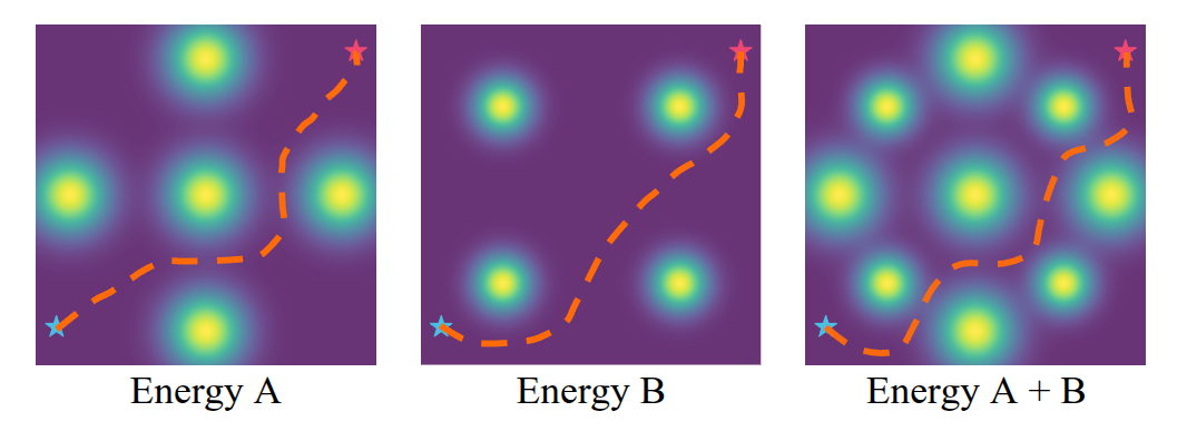
위 그림은 Energy A와 Energy B를 composition해서 새로운 constraint를 ad-hoc하게 추가할 수 있음을 보여준다.

Contribution

1. Potential-based motion planning에 diffusion model을 적용하는 방법을 제안한다.
2. Classical planner와 learning-based motion planner를 비교하여 정확도와 collision check 측면에서의 성능을 보인다.
3. 다양한 motion constraint set을 조합할 수 있는 compositionality를 설명한다.

Method

Potential Function

\[U(q) = U_{\mathrm{att}}(q) + U_{\mathrm{repel}}(q)\]

$U(q)$는 goal state인 $q_e$에는 낮은 potential 값을, collision 상태인 state에는 높은 potential 값을 부여하는 함수이다.

$U_{\mathrm{att}}(q)$는 attraction potential이며, goal state인 $q_e$에는 낮은 potential을 부여하고 goal에서 멀어질수록 높은 potential을 부여한다.

$U_{\mathrm{repel}}(q)$는 repulsive potential이며, 장애물에 가까울수록 높은 값을 부여하고 멀어질수록 낮은 값을 부여한다.

potential function을 정의하면, gradient descent 방식으로 configuration을 다음과 같이 업데이트할 수 있다.

\[q_t = q_{t-1} - \gamma \nabla_q U(q_{t-1})\]

여기서 $\gamma$는 step size이고, $-\nabla_q U$는 potential이 감소하는 방향이다. 즉 현재 configuration에서 goal 쪽으로 이동하면서 obstacle의 높은 potential 영역을 피하도록 업데이트한다.

이 방식의 주된 한계는 local minima에 빠질 수 있다는 점이다. 한 번 local minima에 빠지면 gradient가 더 이상 goal까지의 유효한 방향을 제공하지 못하므로, 경로를 성공적으로 구성하지 못할 수 있다.

$U(q)$는 추가적인 장애물을 통합하는 데 쉬운 접근 방법을 제공한다. motion planning에서는 새로운 obstacle potential $U_{\mathrm{new}}(q)$를 위 수식처럼 더하는 방식으로 확장할 수 있다.

Motion Planning Formulation

\[q_{1:T}^{*} = \arg\min_{q_{1:T}} U_{\theta}(q_{1:T}, q_{\mathrm{st}}, q_e, \mathcal{C})\]

이 논문은 configuration 하나에 대한 potential이 아니라, trajectory level의 potential function $U_{\theta}$를 학습하는 것을 제안한다. $U_{\theta}$는 시작 상태 $q_{\mathrm{st}}$, 목표 상태 $q_e$, 환경 정보 $\mathcal{C}$가 주어졌을 때 trajectory $q_{1:T}$가 얼마나 적절한지를 평가한다.

이를 학습하기 위해 이미 풀린 motion planning 문제들로 구성된 dataset을 사용한다.

\[\mathcal{D} = \{(q_{\mathrm{st}}^i, q_e^i, q_{1:T}^i, \mathcal{C}^i)\}_{i=1}^{M}\]

그리고 EBM(Energy-Based Model) 방식으로 trajectory의 conditional distribution을 다음과 같이 표현한다.

\[\exp\left(-E_{\theta}(q_{1:T} \mid q_{\mathrm{st}}, q_e, \mathcal{C})\right) \propto p(q_{1:T} \mid q_{\mathrm{st}}, q_e, \mathcal{C})\]

즉 좋은 trajectory일수록 낮은 energy를 갖고, 낮은 energy를 갖는 trajectory가 더 높은 확률을 갖도록 학습한다.

따라서 이 dataset으로 학습된 $E_{\theta}$는 성공적인 motion plan에 대해서 낮은 energy를 부여하고, 실패하거나 충돌이 발생하는 trajectory에는 높은 energy를 부여하는 함수가 된다.

즉 EBM의 energy landscape를 직접 설계하는 대신, 최적화로 생성된 motion plan들을 사용해 학습한다. 이때 energy landscape는 denoising diffusion training 방식으로 형성되며, 학습된 모델은 noisy trajectory를 점진적으로 성공적인 trajectory 쪽으로 이동시키는 방향을 제공한다.

구체적으로는 성공적인 motion plan $q_{1:T}^i$에 Gaussian noise $\epsilon$을 섞어 noisy trajectory를 만들고, energy function의 gradient가 이 noise를 제거하는 방향을 학습하도록 한다.

\[\tilde{q}_{1:T}^{i,s} = \sqrt{1 - \beta_s}\, q_{1:T}^i + \sqrt{\beta_s}\, \epsilon\] \[\mathcal{L}_{\mathrm{MSE}} = \left\| \epsilon - \nabla_{q_{1:T}} E_{\theta} \left( \tilde{q}_{1:T}^{i,s}, s, q_{\mathrm{st}}^i, q_e^i, \mathcal{C}^i \right) \right\|_2^2\]

여기서 $\epsilon \sim \mathcal{N}(0, I)$는 Gaussian noise이고, $\beta_s$는 diffusion step $s$에서 적용되는 Gaussian noise corruption 정도를 나타낸다. $s \in {1, 2, \dots, S}$는 denoising diffusion step이며, 보통 $S=100$으로 두어 여러 noise level에서 denoising 방향을 학습한다.

Overall Pipeline

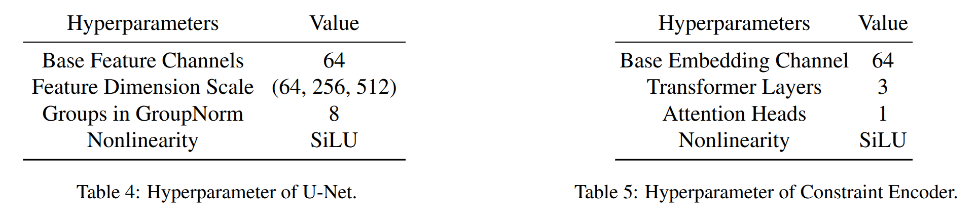
아키텍처는 크게 U-Net 기반 CNN trajectory denoiser와 constraint encoder로 구성된다. U-Net은 noisy trajectory를 입력받아 denoising 방향을 예측하고, constraint encoder는 환경 configuration을 조건 정보로 encoding한다.

Constraint encoder는 Transformer encoder 구조를 사용한다. 정적 환경에서는 장애물 위치들의 집합을 입력으로 받고, 동적 환경에서는 시간에 따라 변화하는 obstacle trajectory들의 집합을 입력으로 받는다.

이때 장애물들은 서로 순서가 중요하지 않아야 하므로 positional embedding은 제거한다. Transformer에서 학습된 class token을 diffusion step의 time embedding과 concatenate한 뒤, 그 결과를 U-Net의 temporal convolution block에 넣어 constraint-aware denoising을 수행한다.

각 모델의 hyperparameter setting은 다음과 같다.

Sampling / Optimization

학습된 diffusion potential function으로부터 motion path를 생성할 때는, 먼저 diffusion step $S$에서 Gaussian noise로 motion path를 초기화한다. 이후 energy function $E_{\theta}$의 gradient를 따라 motion path를 반복적으로 업데이트한다.

\[\epsilon = \nabla_{q_{1:T}} E_{\theta} \left( q_{1:T}^{s}, s, q_{\mathrm{st}}, q_e, \mathcal{C} \right)\] \[q_{1:T}^{s-1} = q_{1:T}^{s} - \gamma \epsilon + \xi, \qquad \xi \sim \mathcal{N}(0, \sigma_s^2 I)\]

Sampling 과정에서는 classifier-free guidance scale을 사용해 조건 정보 $\mathcal{C}$가 energy gradient에 반영되는 정도를 조절한다. 여기서 $\mathcal{C}$는 environment/constraint condition이고, $\gamma$와 $\sigma_s^2$는 diffusion sampling 과정에서 사용하는 상수이다.

Composing Potential Functions

서로 다른 constraint를 학습한 두 energy function $E_{\theta}^{1}(\cdot)$, $E_{\theta}^{2}(\cdot)$가 있을 때, 둘을 단순히 더해서 combined energy function을 만들 수 있다.

\[E^{\mathrm{comb}}(\cdot) = E_{\theta}^{1}(\cdot) + E_{\theta}^{2}(\cdot)\]

이를 $N$개의 constraint로 일반화하면 다음과 같이 쓸 수 있다.

\[E_{\theta}^{\mathrm{comb}}(q_{1:T}, s, q_{\mathrm{st}}, q_e, \mathcal{C}_{1:N}) = \sum_{i=1}^{N} E_{\theta}(q_{1:T}, s, q_{\mathrm{st}}, q_e, \mathcal{C}_i)\]

정적 장애물은 미리 정의된 constraint로 볼 수 있고, 동적 장애물은 시간에 따라 변하는 constraint로 볼 수 있다. 따라서 정적 장애물 $N_1$개와 동적 장애물 $N_2$개가 있을 때 composite diffusion potential function은 다음과 같이 쓸 수 있다.

\[E_{\theta}^{\mathrm{comb}} \left( q_{1:T}, s, q_{\mathrm{st}}, q_e, [\mathcal{C}_{1:N_1}^{s}, \mathcal{C}_{1:N_2}^{d}] \right) = \sum_{i=1}^{N_1} E_{\theta_s}^{i} \left( q_{1:T}, s, q_{\mathrm{st}}, q_e, \mathcal{C}_i^{s} \right) + \sum_{j=1}^{N_2} E_{\theta_d}^{j} \left( q_{1:T}, s, q_{\mathrm{st}}, q_e, \mathcal{C}_{j,1:T}^{d} \right)\]

여기서 $\mathcal{C}_i^{s}$는 $i$번째 static obstacle condition이고, $\mathcal{C}_{j,1:T}^{d}$는 시간에 따라 변하는 $j$번째 dynamic obstacle condition이다.

이렇게 합쳐진 potential function은 두 constraint를 모두 만족하는 trajectory에 낮은 energy를 부여한다.

만약 각 constraint가 서로 독립적이라면, 이렇게 composition한 potential은 여러 constraint를 결합한 ground-truth potential로 볼 수 있다.

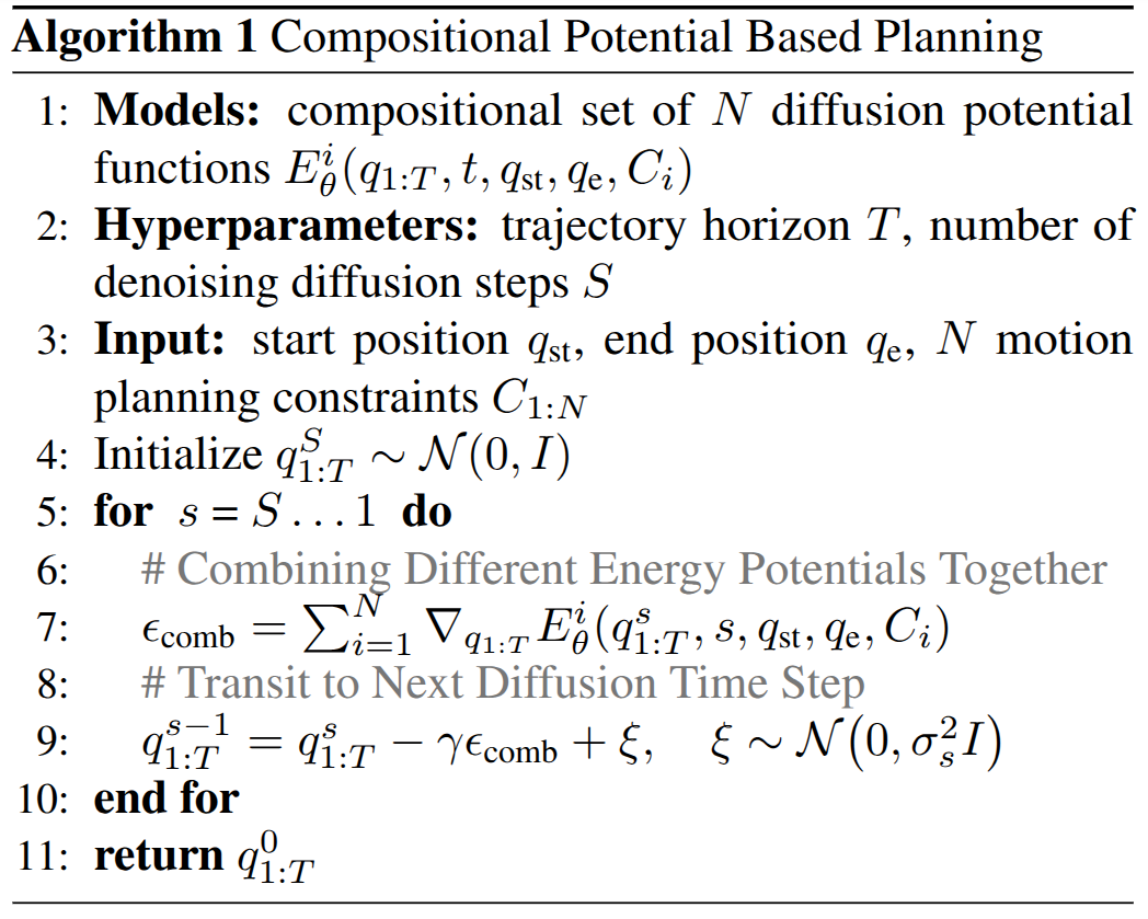
실제 응용 관점에서 모든 제약조건의 조합을 하나의 모델로 미리 학습하는 것은 어렵다. 테스트 환경에서는 학습 때 보지 못한 새로운 제약조건의 조합이 등장할 수 있기 때문이다. 이 방식은 새로운 constraint에 해당하는 energy function을 계속 추가하고 composition할 수 있으므로, 이런 문제를 완화할 수 있다. Algorithm 1은 이러한 composition 기반 sampling 절차를 설명한다.

합쳐진 potential function $E^{\mathrm{comb}}$에서 sample하기 위해서는 다음과 같이 combined gradient를 사용한다.

\[\epsilon_{\mathrm{comb}} = \nabla_{q_{1:T}} \left( E_{\theta}^{1}(q_{1:T}^{s}, s, q_{\mathrm{st}}, q_e, \mathcal{C}_1) + E_{\theta}^{2}(q_{1:T}^{s}, s, q_{\mathrm{st}}, q_e, \mathcal{C}_2) \right)\] \[q_{1:T}^{s-1} = q_{1:T}^{s} - \gamma \epsilon_{\mathrm{comb}} + \xi, \qquad \xi \sim \mathcal{N}(0, \sigma_s^2 I)\]

Refinement with Warm-start Denoising

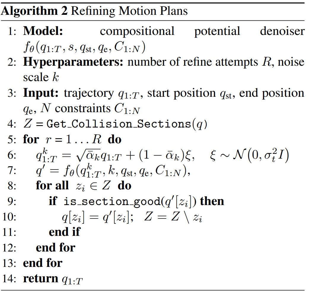
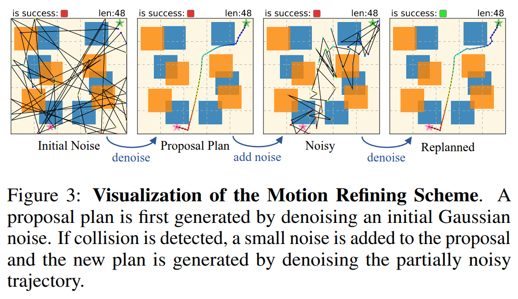
예측된 motion plan은 우연히 일부 section에서 constraint를 침해할 수 있다. Classical motion planner나 learning-based motion planner들은 이런 문제를 다루기 위해 trajectory를 정제(refinement)하는 절차를 제공한다.

Diffusion potential fields에서는 반대로, collision이 있는 기존 trajectory를 noisy trajectory로 perturbing한 뒤 다시 denoising하는 방식으로 trajectory를 수정한다. 먼저 forward process의 임의의 $k$ step을 사용해 기존 trajectory $q_{1:T}$에 noise를 추가한다.

\[q_{1:T}^{k} = \sqrt{\bar{\alpha}_k}\, q_{1:T} + \sqrt{1 - \bar{\alpha}_k}\, \xi, \qquad \xi \sim \mathcal{N}(0, I)\]

그 다음 일반적인 denoising 과정을 사용해 새로운 motion plan $q’_{1:T}$를 생성한다.

\[q'_{1:T} = f_{\theta}(q_{1:T}^{k}, k, q_{\mathrm{st}}, q_e, \mathcal{C}_{1:N})\]

만약 기존 trajectory $q_{1:T}$ 안에 constraint를 만족하지 않는 section이 있다면, 해당 section에 대응되는 구간을 $q’_{1:T}$에서 가져와 교체한다. 이때 교체되는 section은 전체 trajectory와 coherent해야 하고 collision-free해야 한다.

이 refinement 과정은 원하는 trajectory를 찾을 때까지 반복할 수 있다. Warm-start denoising scheme은 처음부터 새 trajectory를 생성하는 것보다 빠른 replanning을 가능하게 하고, 동시에 기존 plan의 전체적인 형태를 유지할 수 있게 한다.

Algorithm 2는 이러한 refinement pipeline을 정리한 것이다.

아래 그림은 refinement 과정과 관련된 예시이다.

Probabilistic Completeness

Probabilistic completeness를 다루기 위해, diffusion potential model의 output distribution을 $\mathcal{D}_0$라고 두고, 이에 대한 probability density function을 $f_{\theta}(q_{1:T})$로 정의한다.

제약 $\mathcal{C}$를 만족하는 feasible trajectory를 $q_{1:T}^{\mathcal{C}}$라고 하자. 또한 이 trajectory 주변의 $\tau$-neighborhood를 $B_{\tau}(q_{1:T}^{\mathcal{C}})$라고 두면,

\[B_{\tau}(q_{1:T}^{\mathcal{C}}) = \left\{ x \mid \left\|x - q_{1:T}^{\mathcal{C}}\right\| \le \tau \right\}\]

이다. 이 neighborhood 안에서 모델이 trajectory를 샘플할 확률을 $P_{\tau}$라고 하면,

\[P_{\tau} = \int_{B_{\tau}(q_{1:T}^{\mathcal{C}})} f_{\theta}(x)\,dx > 0\]

로 쓸 수 있다.

$A_n$을 $n$개의 샘플링된 trajectory 중 적어도 하나가 $B_{\tau}(q_{1:T}^{\mathcal{C}})$ 안에 속하는 사건이라고 하자. 즉, $n$개의 후보 trajectory 중 하나 이상이 제약 $\mathcal{C}$를 만족하는 feasible trajectory 근방에 들어가는 사건이다.

각 샘플이 독립적으로 생성된다고 보면,

\[\mathbb{P}(A_n) = 1 - (1 - P_{\tau})^n\]

이고, $P_{\tau} > 0$이므로 샘플 수가 무한대로 증가하면

\[\lim_{n \to \infty} \mathbb{P}(A_n) = 1\]

이 된다. 따라서 diffusion potential model이 feasible trajectory 주변에 non-zero probability mass를 가진다면, 샘플 수가 충분히 증가했을 때 제약을 만족하는 trajectory를 찾을 확률은 1에 수렴한다. 이러한 의미에서 이 방법은 probabilistically complete하다고 볼 수 있다.

Experiments

실험 설정

실험은 2D point robot부터 14 DoF dual-arm setting까지 난이도를 점진적으로 높여 구성한다.

Environment	Configuration space	설명
Static Maze2D	2D $(x, y)$	2D workspace에서 point robot이 움직이는 환경이다. 장애물은 고정되어 있다.
Dynamic Maze2D	2D $(x, y)$	Maze2D와 동일한 point robot 환경이지만, 장애물이 randomly generated linear trajectory를 따라 움직인다.
KUKA	7D joint state	3D tabletop workspace에서 7 DoF KUKA arm이 움직이는 환경이다. start/goal은 KUKA arm의 7D joint state로 주어진다.
Dual KUKA	14D joint state	두 개의 KUKA arm이 tabletop 위에 나란히 배치되어 동시에 움직이는 환경이다. start/goal은 두 arm의 joint state를 합친 14 DoF state로 주어진다.

비교 대상

비교 대상은 method의 성격에 따라 다음과 같이 나눌 수 있다.

구분	비교 방법	비교 의도
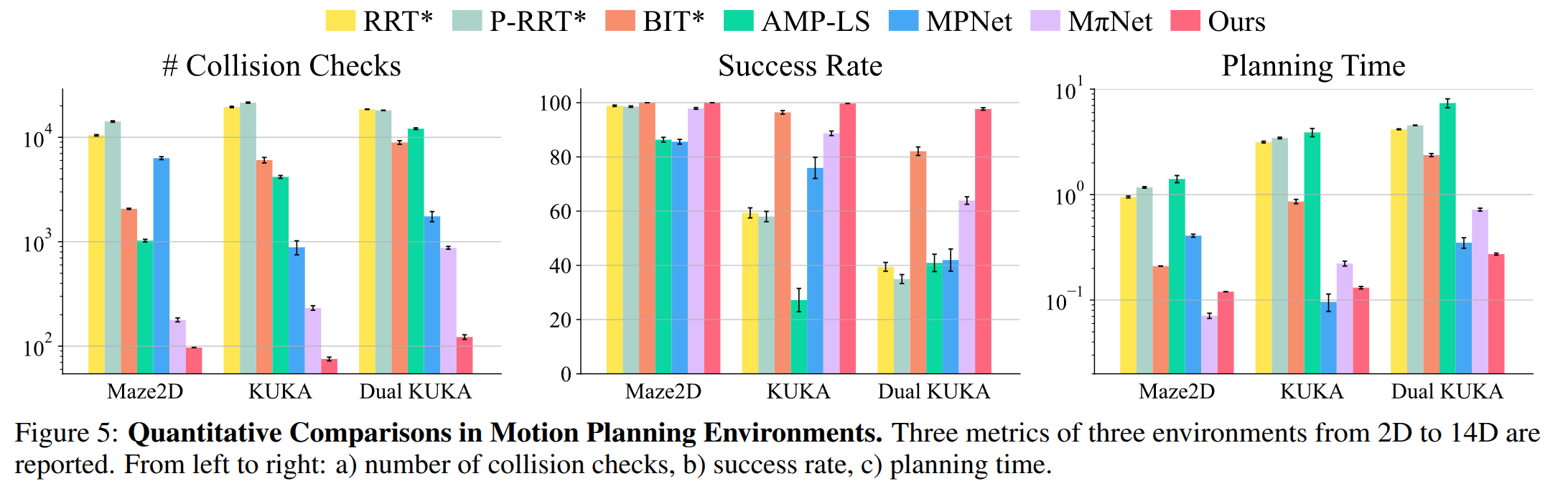
Classical planning baselines	RRT*, P-RRT*, BIT*, SIPP	sampling/search 기반 planner와 성공률, planning time, collision check 수를 비교
Classical potential-based baseline	RMP	전통적인 potential-based method와 비교
Learning-based baselines	MPNet, M$\pi$Net, AMP-LS	기존 학습 기반 motion planner와 generalization 및 planning 효율성 비교

실험 결과

아래 결과는 Maze2D, KUKA, Dual KUKA 환경에서 collision check 수, success rate, planning time을 비교한 것이다.

저자가 제시한 한계 및 추가제안

1. 생성된 motion trajectory는 collision-free 측면에서는 정확할 수 있지만, 종종 sub-optimal할 수 있다. 예를 들어 더 짧은 path가 존재하더라도 모델이 반드시 최단 경로를 선택하는 것은 아니다. 이 부분은 goal에 더 빠르게 도달하도록 유도하는 reach-related potential을 추가하면 어느 정도 완화할 수 있을 것으로 보인다.
2. Potential을 조합하는 방식은 조합되는 모델의 수에 비례하여 계산량이 증가한다. 즉, 더 많은 constraint나 obstacle-specific potential을 추가할수록 sampling 과정에서 더 많은 연산 자원이 필요하다. 이는 서로 다른 potential들이 하나의 네트워크 내부에서 feature를 공유하도록 설계함으로써 완화할 수 있다.