[논문리뷰] Generative Modeling via Drifting
논문 정보
- Title: Generative Modeling via Drifting (arXiv 2026)
- Authors: Mingyang Deng, He Li, Tianhong Li, Yilun Du, Kaiming He
- Links: Project, Paper, Code
한 줄 요약
- diffusion이나 flow matching에서 data distribution에 가까워지기 위해 반복적으로 noise를 제거하거나 vector field를 따라 sample을 이동시키는 과정을, inference time에는 한 번의 forward pass로 수행할 수 있게 만든 generative modeling 방법
문제 정의
Generative model은 prior sample $z \sim p_z$를 generator $f_{\theta}$로 data space에 mapping한다.
\[z \sim p_z, \qquad x = f_{\theta}(z)\]이때 생성된 distribution은 pushforward distribution $q_{\theta}$로 표현된다.
\[q_{\theta} = (f_{\theta})_{\sharp} p_z\]따라서 목표는 $q_{\theta}$가 실제 data distribution $p_{\mathrm{data}}$와 가까워지도록 $f_{\theta}$를 학습하는 것이다.
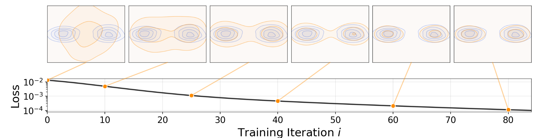
위 그림은 training이 진행될수록 generator가 만든 pushforward distribution이 data distribution에 가까워지는 과정을 보여준다. 아래 loss curve는 iteration이 증가할수록 두 distribution 사이의 loss가 낮아지는 것을 나타낸다.
기존 방식의 한계
기존 generative model 중 diffusion-based model과 flow-based model은 prior distribution에서 data distribution으로 sample을 이동시키는 과정을 반복적으로 수행한다.
| 구분 | 대표 연구 | 핵심 방식 | 한계 |
|---|---|---|---|
| Diffusion-based model | Deep Unsupervised Learning using Nonequilibrium Thermodynamics, Denoising Diffusion Probabilistic Models, Score-Based Generative Modeling through Stochastic Differential Equations | noise를 점진적으로 제거하면서 sample을 data distribution 쪽으로 이동시킨다. | inference time에 여러 step의 neural network evaluation이 필요하다. |
| Flow-based model | Flow Matching for Generative Modeling, Flow Straight and Fast, Stochastic Interpolants | vector field를 따라 sample을 data distribution 쪽으로 이동시킨다. | SDE/ODE dynamics를 수치적으로 풀기 위해 여러 step update가 필요할 수 있다. |
| Step reduction | distillation-based method, from-scratch one-step generator | inference step을 줄이기 위해 반복적인 SDE/ODE dynamics를 training 과정 안에 포함시키려 한다. | 별도의 distillation 과정이나 one-step generator training이 필요하다. |
| GAN 계열 one-step generator | GAN | single forward pass로 sample을 생성하지만 adversarial optimization을 사용한다. | training instability나 mode collapse 문제가 발생할 수 있다. |
핵심 아이디어
Drifting model은 복잡한 pushforward map을 inference time에 여러 step으로 나누어 수행하는 대신, training time에 학습시키는 방식이다. 이를 통해 diffusion이나 flow matching에서 필요한 iterative inference 절차를 제거하고, 학습된 generator의 single forward pass로 sample을 생성할 수 있게 한다.
이를 위해 저자는 drifting field라는 개념을 정의한다. Drifting field는 generated distribution과 data distribution의 차이에 의존해 sample들이 어느 방향으로 움직여야 하는지를 나타내는 field이다. 두 distribution이 match되면 더 이상 이동시킬 방향이 없으므로 drifting field는 0이 된다.
Method
Pushforward Distribution
Generator를 다음과 같은 mapping으로 둔다.
\[f : \mathbb{R}^{C} \to \mathbb{R}^{D}\]입력은 noise $\epsilon \sim p_{\epsilon}$이고, output은 data space의 sample $\mathbf{x} = f(\epsilon) \in \mathbb{R}^{D}$이다. 이때 input dimension $C$와 output dimension $D$는 서로 달라도 된다.
network output의 distribution을 $q$라고 두면 다음과 같이 쓸 수 있다.
\[\mathbf{x} = f(\epsilon) \sim q\]$q$는 $p_{\epsilon}$이 $f$에 의해 밀려서 만들어진 pushforward distribution이다.
\[q = f_{\sharp}p_{\epsilon}\]여기서 $\sharp$는 $f$에 의해 유도되는 pushforward를 의미한다.
neural network training은 반복적으로 진행되므로, training 과정은 model sequence ${f_i}$를 만든다고 볼 수 있다. 마찬가지로 각 training iteration $i$에 대응되는 pushforward distribution sequence ${q_i}$도 정의할 수 있다.
\[q_i = [f_i]_{\sharp}p_{\epsilon}\]training이 진행될수록 $q_i$는 점진적으로 data distribution $p_{\mathrm{data}}$와 match되도록 학습된다.
Drifting Field for Training
training iteration이 진행되면서 generator $f_i$가 $f_{i+1}$로 업데이트되면, 같은 noise $\epsilon$에서 생성되는 sample도 함께 이동한다.
\[\mathbf{x}_{i+1} = \mathbf{x}_i + \Delta \mathbf{x}_i\]여기서 $\Delta \mathbf{x}_i$는 다음과 같이 정의된다.
\[\Delta \mathbf{x}_i := f_{i+1}(\epsilon) - f_i(\epsilon)\]즉 $\Delta \mathbf{x}_i$는 generator $f$의 parameter update로 인해 발생하는 sample의 차이값이다. 이처럼 training 과정에서 $f$가 업데이트되면서 generated sample $\mathbf{x}$가 이동하는 현상을 이 논문에서는 drift로 정의한다.
drifting field는 현재 sample $\mathbf{x}$가 주어졌을 때, 그 sample이 이동해야 하는 방향 $\Delta \mathbf{x}$를 계산하는 함수로 볼 수 있다.
\[V_{p,q}(\cdot) : \mathbb{R}^{D} \to \mathbb{R}^{D}\]앞의 training iteration은 drifting field를 사용해 다음과 같이 다시 쓸 수 있다.
\[\mathbf{x}_{i+1} = \mathbf{x}_i + V_{p,q_i}(\mathbf{x}_i)\]여기서 $p$는 data distribution $p_{\mathrm{data}}$를 줄여 쓴 것이고, $q_i$는 training iteration $i$에서의 current generated distribution을 의미한다.
\[\mathbf{x}_i = f_i(\epsilon) \sim q_i\]drifting 이후 sample은 다음 iteration의 generated distribution에 대응된다.
\[\mathbf{x}_{i+1} \sim q_{i+1}\]Proposition 1. Drifting field는 anti-symmetric property를 갖는다.
\[V_{p,q}(\mathbf{x}) = -V_{q,p}(\mathbf{x}), \qquad \forall \mathbf{x}\]또한 generated distribution과 data distribution이 같아져 $q = p$가 되면, drifting field는 0이 된다.
\[q = p \Rightarrow V_{p,q}(\mathbf{x}) = 0, \qquad \forall \mathbf{x}\]직관적으로는 $p$와 $q$의 위치를 바꾸면, sample을 이동시켜야 하는 방향만 반대로 바뀌어야 한다. 따라서 같은 위치 $\mathbf{x}$에서 $V_{p,q}$와 $V_{q,p}$는 부호만 다른 field가 된다.
또한 $p$와 $q$가 match되면 더 이상 한 distribution을 다른 distribution 쪽으로 이동시킬 필요가 없으므로 drift는 0이 된다. 다만 converse implication은 일반적으로 성립하지 않는다. 즉 $V_{p,q} = 0$이라고 해서 항상 $q = p$라고 말할 수는 없다.
Training Objective
$f_{\theta}$를 parameter $\theta$를 갖는 neural network라고 두고, noise $\epsilon \sim p_{\epsilon}$에 대해 generated sample을 $\mathbf{x} = f_{\theta}(\epsilon)$ 이라 한다.
앞에서 정의한 drifting field를 사용하면, 현재 generator의 output을 data distribution 쪽으로 이동시킨 target generator를 다음처럼 생각할 수 있다.
\[f_{\mathrm{target}}(\epsilon) = f_{\theta}(\epsilon) + V_{p,q_{\theta}}\!\left(f_{\theta}(\epsilon)\right)\]이 식은 training 과정에서 fixed-point iteration을 유도한다. 즉 training iteration $i$에서 다음을 만족하는 새로운 network $f_{\theta_{i+1}}$를 찾는 방식으로 볼 수 있다.
\[f_{\theta_{i+1}}(\epsilon) \leftarrow f_{\theta_i}(\epsilon) + V_{p,q_{\theta_i}}\!\left(f_{\theta_i}(\epsilon)\right)\]이를 loss function으로 바꾸면 다음과 같이 쓸 수 있다.
\[\mathcal{L} = \mathbb{E}_{\epsilon} \left[ \left\| f_{\theta}(\epsilon) - \operatorname{stopgrad} \!\left( f_{\theta}(\epsilon) + V_{p,q_{\theta}}\!\left(f_{\theta}(\epsilon)\right) \right) \right\|^2 \right]\]여기서 stop-gradient operation은 target이 되는 frozen state를 제공한다. 즉 현재 network output에 drifting field를 더해 만든 target을 고정해 두고, $f_{\theta}$가 그 target에 가까워지도록 학습한다.
Designing the Drifting Field
$V_{p,q}$는 $p$와 $q$ 두 distribution에 의존하므로, 실제로 계산 가능한 형태를 얻기 위해 추가적인 정의가 필요하다. 이를 위해 논문에서는 kernel-like function $\mathcal{K}(\cdot,\cdot,\cdot)$를 사용해 drifting field를 다음과 같이 정의한다.
\[V_{p,q}(\mathbf{x}) = \mathbb{E}_{\mathbf{y}^{+} \sim p} \mathbb{E}_{\mathbf{y}^{-} \sim q} \left[ \mathcal{K}(\mathbf{x}, \mathbf{y}^{+}, \mathbf{y}^{-}) \right] \tag{1}\]$\mathcal{K}$는 세 개의 sample point 사이의 interaction을 계산하는 함수로 볼 수 있으며, 선택적으로 $p$와 $q$에 의존할 수 있다. 이 framework는 하나의 특정 kernel만 가정하지 않고, 비교적 넓은 class의 function $\mathcal{K}$를 지원한다.
직관적으로 $V$는 attraction과 repulsion으로부터 유도된 field로 볼 수 있다. Data distribution 쪽으로는 sample을 끌어당기고, current generated distribution 안에서는 sample들이 적절히 퍼지도록 만드는 방식이며, 이는 mean-shift 방식에서 영감을 받은 해석이다. 마찬가지로 $p = q$가 되면 이동시킬 방향이 사라지므로 $V$는 0이 된다.
구체적으로 이 논문에서는 다음과 같은 attraction field와 repulsion field를 사용한다.
\[\begin{aligned} V_p^{+}(\mathbf{x}) &:= \frac{1}{Z_p(\mathbf{x})} \mathbb{E}_{p} \!\left[ k(\mathbf{x},\mathbf{y}^{+}) \left( \mathbf{y}^{+} - \mathbf{x} \right) \right], \\[6pt] V_q^{-}(\mathbf{x}) &:= \frac{1}{Z_q(\mathbf{x})} \mathbb{E}_{q} \!\left[ k(\mathbf{x},\mathbf{y}^{-}) \left( \mathbf{y}^{-} - \mathbf{x} \right) \right]. \end{aligned} \tag{2}\]여기서 $Z_p(\mathbf{x})$와 $Z_q(\mathbf{x})$는 normalization factor이다.
\[\begin{aligned} Z_p(\mathbf{x}) &:= \mathbb{E}_{p} \!\left[ k(\mathbf{x},\mathbf{y}^{+}) \right], \\[4pt] Z_q(\mathbf{x}) &:= \mathbb{E}_{q} \!\left[ k(\mathbf{x},\mathbf{y}^{-}) \right]. \end{aligned} \tag{3}\]이는 직관적으로 $\mathbf{y} - \mathbf{x}$ 차이 vector의 weighted mean을 계산하는 것이다. 최종 drifting field는 다음처럼 attraction에서 repulsion을 빼는 방식으로 정의된다.
\[V_{p,q}(\mathbf{x}) := V_p^{+}(\mathbf{x}) - V_q^{-}(\mathbf{x}) \tag{4}\]앞에서 정의한 두 식을 합치면 다음과 같은 형태가 된다.
\[V_{p,q}(\mathbf{x}) = \frac{1}{Z_p(\mathbf{x})Z_q(\mathbf{x})} \mathbb{E}_{p,q} \!\left[ k(\mathbf{x},\mathbf{y}^{+}) k(\mathbf{x},\mathbf{y}^{-}) \left( \mathbf{y}^{+} - \mathbf{y}^{-} \right) \right] \tag{5}\]이는 positive sample $\mathbf{y}^{+}$가 있는 방향으로 sample을 끌어당기고, negative sample $\mathbf{y}^{-}$가 만드는 방향은 빼는 형태로 작동한다. 이때 weight는 두 개의 kernel $k(\mathbf{x},\mathbf{y}^{+})$, $k(\mathbf{x},\mathbf{y}^{-})$와 normalization factor $Z_p(\mathbf{x})Z_q(\mathbf{x})$로부터 jointly 계산된다.
결국 식 (5)는 식 (1)의 구체적인 instantiation으로 볼 수 있다. 이 형태에서는 $V$가 anti-symmetric하다는 점도 비교적 쉽게 확인할 수 있다. 다만 이 방법이 항상 attraction과 repulsion으로 분해되어야 하는 것은 아니다. 일반적으로 필요한 조건은 $p = q$일 때 $V = 0$이 되는 것이다.
kernel $k(\cdot,\cdot)$는 두 sample 사이의 유사성을 측정하는 함수이다. 이 논문에서는 다음 형태를 사용한다.
\[k(\mathbf{x},\mathbf{y}) = \exp\!\left( -\frac{1}{\tau} \|\mathbf{x}-\mathbf{y}\|_2 \right) \tag{6}\]여기서 $\tau$는 temperature이고, $|\cdot|_2$는 $\ell_2$ distance이다. 식 (5)에서는 normalization factor가 함께 들어가므로, normalized kernel을 다음처럼 볼 수 있다.
\[\tilde{k}(\mathbf{x},\mathbf{y}) := \frac{1}{Z} k(\mathbf{x},\mathbf{y})\]실제 구현에서는 $\tilde{k}$를 softmax operation으로 계산한다. 이때 logit은 $-\frac{1}{\tau}|\mathbf{x}-\mathbf{y}|_2$로 주어지고, softmax는 $\mathbf{y}$에 대해 계산된다.
추가로 논문에서는 batch 안의 generated sample set ${\mathbf{x}}$에 대해서 한 번 더 softmax normalization을 적용한다. 이는 실제 성능을 조금 개선하며, 이렇게 추가된 normalization은 최종 $V$의 anti-symmetric property를 바꾸지 않는다.
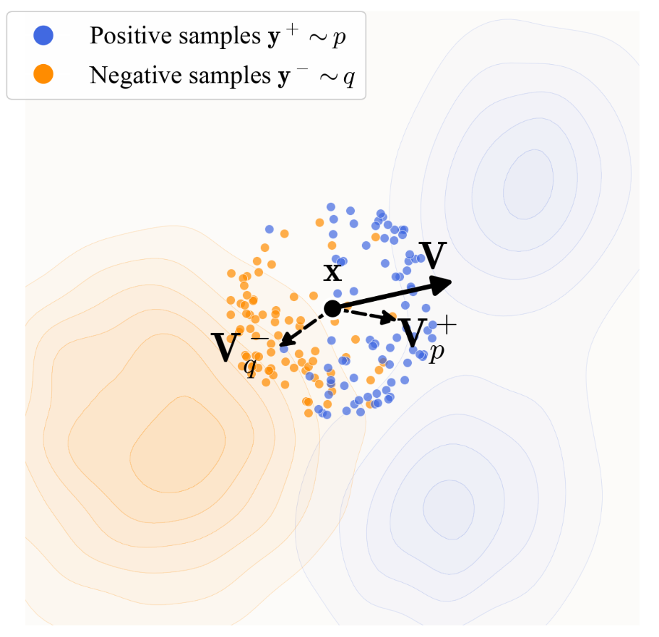
위 그림은 positive sample $\mathbf{y}^{+} \sim p$가 attraction field $V_p^{+}$를 만들고, negative sample $\mathbf{y}^{-} \sim q$가 repulsion field $V_q^{-}$를 만드는 과정을 보여준다. 최종 drifting field $V$는 이 두 방향의 차이로 결정된다.
이 loss의 값은 drifting field $V$의 squared norm을 최소화하는 것과 같은 의미로 볼 수 있다.
\[\mathbb{E}_{\epsilon} \left[ \left\| V\!\left(f_{\theta}(\epsilon)\right) \right\|^2 \right] \tag{7}\]다만 이는 loss의 값이 $|V|^2$와 같다는 의미이지, $|V|^2$를 직접 미분한다는 뜻은 아니다. stop-gradient 때문에 gradient는 target 바깥쪽 $f_{\theta}$로만 흐르며, $f_{\theta}$는 고정된 drifted target $f_{\theta} + V$ 쪽으로 당겨진다.
따라서 이 loss는 $|V|^2$를 줄이도록 학습한다. 이상적으로는 $V \approx 0$이면 $q \approx p$가 되기를 기대할 수 있다. 하지만 이 implication은 임의의 $V$에 대해 항상 성립하지는 않는다. 논문에서는 경험적으로 $|V|^2$가 감소할수록 generation quality가 좋아지는 경향을 관찰했고, kernelized construction에서는 zero-drift condition이 $(p,q)$에 많은 bilinear constraint를 부여하여 mild non-degeneracy assumption 아래에서 $p$와 $q$가 근사적으로 match되도록 만든다고 설명한다.
stochastic training에서는 empirical mean을 사용해 $V$를 추정한다. 각 training step에서 noise $\epsilon \sim p_{\epsilon}$를 여러 개 뽑고, 이를 generator에 통과시켜 generated sample batch $\mathbf{x} = f_{\theta}(\epsilon) \sim q$를 만든다. 이 generated sample들은 같은 batch 안에서 negative sample $\mathbf{y}^{-} \sim q$로 사용된다. 반면 positive sample은 data distribution에서 $N_{\mathrm{pos}}$개의 data point를 뽑아 $\mathbf{y}^{+} \sim p_{\mathrm{data}}$로 사용한다.
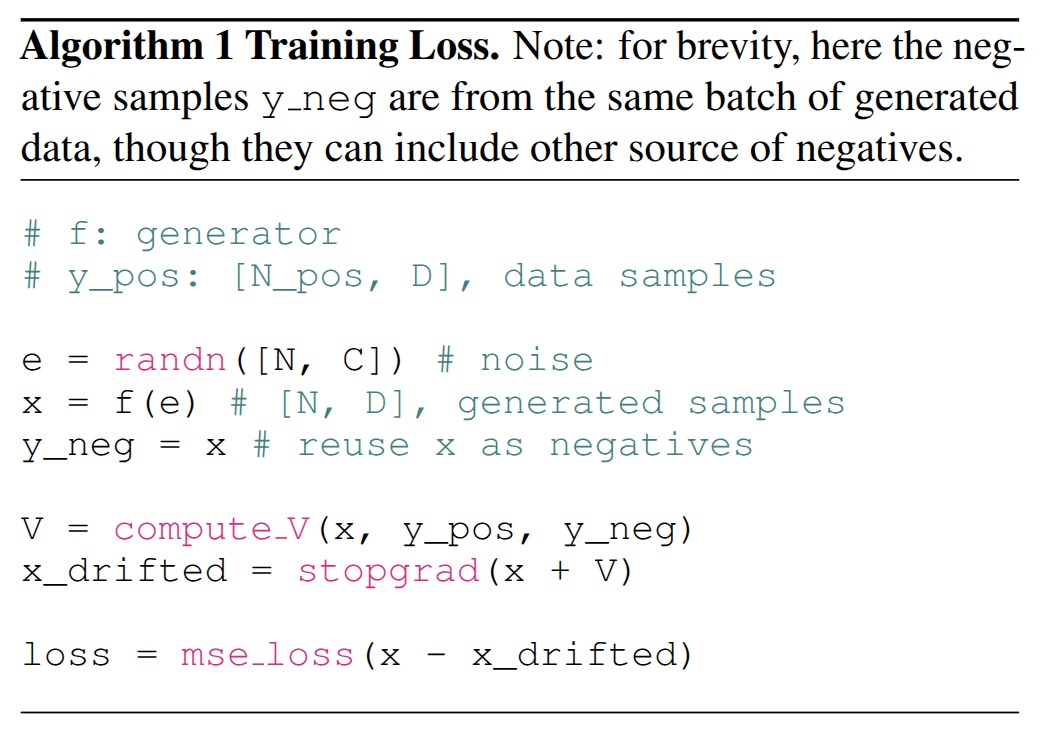
위 알고리즘은 noise에서 generated sample을 만들고, 같은 batch의 generated sample을 negative sample로 재사용한 뒤, positive sample과 함께 $V$를 계산해 drifted target을 만드는 training loss 계산 과정을 보여준다.
다만 stop-gradient formulation에서는 solver가 $V$를 통해 직접 back-propagation을 수행하지 않는다. $V$는 $q_{\theta}$에 의존하고, distribution을 통한 back-propagation은 non-trivial하기 때문이다. 대신 이 objective는 $\mathbf{x} = f_{\theta}(\epsilon)$를 현재 iteration에서 frozen된 drifted version, 즉 $\mathbf{x} + \Delta \mathbf{x}$ 쪽으로 이동시키는 방식으로 목적함수를 간접적으로 최소화한다.
Feature Space
앞의 loss는 raw data space에서 정의했지만, feature extractor $\phi$를 사용하면 feature space에서도 같은 방식으로 쓸 수 있다.
\[\mathbb{E} \left[ \left\| \phi(\mathbf{x}) - \operatorname{stopgrad} \!\left( \phi(\mathbf{x}) + V\!\left(\phi(\mathbf{x})\right) \right) \right\|^2 \right]\]Relation to Perceptual Loss
이 feature-space loss는 perceptual loss와 관련이 있지만 개념적으로는 다르다. Perceptual loss는 보통 다음과 같이 target image $\mathbf{x}_{\mathrm{target}}$와의 feature distance를 줄인다.
\[\left\| \phi(\mathbf{x}) - \phi(\mathbf{x}_{\mathrm{target}}) \right\|_2^2\]즉 regression target은 $\phi(\mathbf{x}{\mathrm{target}})$이고, 이를 위해 $\mathbf{x}$와 $\mathbf{x}{\mathrm{target}}$의 pairing이 필요하다. 반면 drifting의 feature-space loss에서 regression target은 $\phi(\mathbf{x}) + V(\phi(\mathbf{x}))$이다.
Classifier-Free Guidance
Drifting framework는 classifier-free guidance도 기본적으로 지원한다. Class label $c$가 condition으로 주어졌을 때, 수식적으로는 target distribution을 다음처럼 바꾸면 된다.
\[\tilde{q}(\,\cdot \mid c\,) \triangleq (1-\gamma)\, q_{\theta}(\,\cdot \mid c\,) + \gamma\, p_{\mathrm{data}}(\,\cdot \mid \varnothing)\]여기서 $\gamma \in [0,1)$는 conditional 생성 분포 $q_{\theta}(\,\cdot \mid c\,)$와 unconditional data distribution $p_{\mathrm{data}}(\,\cdot \mid \varnothing)$를 섞는 비율을 조절한다.
equilibrium 관점에서는 guided target이 conditional data distribution에 맞춰지도록 $q_{\theta}(\,\cdot \mid c\,)$를 조정하는 것으로 볼 수 있다.
이를 정리하면 다음과 같이 쓸 수 있다.
\[q_{\theta}(\,\cdot \mid c\,) = \alpha\, p_{\mathrm{data}}(\,\cdot \mid c\,) - (\alpha-1)\, p_{\mathrm{data}}(\,\cdot \mid \varnothing)\]여기서 $\alpha = \frac{1}{1-\gamma}$이다.
실제로는 unconditional data distribution $p_{\mathrm{data}}(\,\cdot \mid \varnothing)$에서 추가 negative example을 sampling하는 방식으로 구현된다. 또한 $q_{\theta}(\,\cdot \mid c\,)$는 class-conditional network $f_{\theta}(\cdot \mid c)$에 대응된다.
Experiments
실험 설정
| 항목 | 설정 |
|---|---|
| Image generation task | ImageNet 256x256 |
| Tokenizer | SD-VAE latent space 사용 |
| Latent shape | 32x32x4 |
| Architecture | DiT-like architecture |
| Input | 32x32x4-dimensional Gaussian noise $\epsilon$ |
| Output | input과 같은 32x32x4 latent representation |
| Conditioning | CFG conditioning 사용 |
| Normalization | adaLN-zero 사용 |
| Feature extractor | self-supervised pre-trained ResNet-style encoder 사용. MoCo, SimCLR 기반 encoder를 주로 사용 |
| Feature extraction | pixel-space encoder를 쓸 때는 VAE decoder로 latent output을 pixel space로 복원한 뒤 feature 추출 |
| Multi-scale feature | ResNet-style model의 여러 stage feature map에서 drifting loss를 계산한 뒤 합침 |
| Additional encoder | latent-space pre-trained MAE encoder도 실험 |
| Pixel-space generation | 지원함. 이 경우 $\epsilon,\mathbf{x} \in \mathbb{R}^{256 \times 256 \times 3}$, patch size는 16, $\phi$는 pixel space에 직접 적용 |
Robotic Control
논문에서는 drifting을 image generation뿐 아니라 robotic control에도 적용한다. 구체적으로 diffusion policy에 drifting 방식을 적용하고, 기존 Diffusion Policy의 100 NFE 설정과 Drifting Policy의 1 NFE 설정을 비교한다.
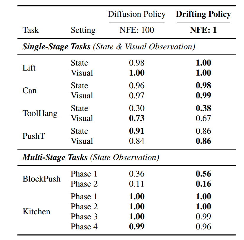
위 결과는 Drifting Policy가 1 NFE만 사용하면서도 여러 robotic control task에서 100 NFE Diffusion Policy와 비슷하거나 더 높은 success rate를 보일 수 있음을 보여준다.
Discussion
이 논문은 $q = p$이면 $V = 0$이 된다는 방향을 보인다. 그러나 반대 방향, 즉 $V \to 0$이면 $q \to p$가 되는지는 일반적으로 이론적으로 보장되지 않는다.
논문에서 설계한 drifting field $V$는 empirical하게 좋은 성능을 보이지만, 어떤 조건에서 $V \to 0$이 실제로 $q \to p$를 의미하는지는 아직 명확하지 않다. 따라서 drifting field의 설계와 zero-drift condition이 distribution matching을 얼마나 강하게 보장하는지는 중요한 논의 지점으로 남는다.
실용적인 관점에서도 현재 제안된 drifting modeling은 효과적인 instantiation이지만, 여러 설계 선택이 아직 sub-optimal일 수 있다. 예를 들어 drifting field와 kernel의 설계, feature encoder 선택, generator architecture는 모두 앞으로 더 탐색될 수 있는 부분이다.
더 넓은 관점에서 보면, 이 논문은 iterative neural network training 자체를 distribution evolution의 mechanism으로 재해석한다. 이는 diffusion이나 flow-based model이 differential equation을 통해 distribution의 변화를 정의하는 것과 대비된다. 저자는 이러한 관점이 앞으로 다른 형태의 training-time distribution evolution 방법을 탐색하는 데 도움이 될 수 있다고 본다.
한계 및 아쉬운 점
1. 2.
내가 이해한 핵심
-