Reinforcement Learning 7 - Distributional Reinforcement Learning

00_Distributional RL

Distributional Reinforcement Learning은 즉각적인 reward의 분포만이 아니라, discounted return이라는 확률변수의 확률분포를 학습한다. Reward, transition, policy action이 모두 확률적일 수 있으므로 return도 random variable이 된다.

Random Return

policy $\pi$에서 $X_0=x, A_0=a$로 시작한다고 하자. 이 조건부 trajectory의 discounted return을 다음과 같이 정의한다.

\[Z^\pi(x,a)=\sum_{t=0}^{\infty}\gamma^t R(X_t,A_t)\]

여기서 $Z^\pi(x,a)$는 고정된 값이 아니라 trajectory의 randomness에 따라 달라지는 random return이다.

Action-value Distribution

기존 강화학습은 이 random return의 평균만 사용하여 action value를 정의한다.

\[Q^\pi(x,a)=\mathbb{E}[Z^\pi(x,a)]\]

기존 RL은 $Q^\pi$라는 mean을 학습하고, Distributional RL은 $Z^\pi$의 전체 확률분포, 즉 action-value distribution을 학습한다.

Distributional Bellman Equation

먼저 Bellman expectation equation는 다음과 같이 표현이 가능하다.

\[Q^\pi(x,a)=\mathbb{E}[R(x,a)+\gamma Q^\pi(x',a')]\]

이를 return의 분포에 대해 쓰면 distributional Bellman equation이 된다.

\[Z^\pi(x,a)\mathrel{\overset{D}{=}}R(x,a)+\gamma Z^\pi(x',a')\]

여기서 $\mathrel{\overset{D}{=}}$는 두 확률변수가 equality in distribution을 만족한다는 뜻이다.

여기서 임의의 policy $\pi$를 따를때 $Z^\pi(x’,a’)$는 현재 reward $R(x,a)$와 다음 state, action $(x’,a’)$에서의 $Z^\pi(x’,a’)$으로 표현된다.

Distributional Bellman Operator

위의 Distributional Bellman equation에서 우변의 연산을 하나의 mapping으로 정의한 것이 Distributional Bellman operator이다. 이를 다음과 같이 표현할 수 있다.

\[(\mathcal{T}^\pi Z)(x,a) \mathrel{\overset{D}{=}} R(x,a)+\gamma Z(x',a')\]

여기서 $\mathcal{T}^\pi$는 임의의 return distribution $Z$를 입력으로 받아, 현재 reward와 다음 상태의 return distribution을 이용해 새로운 return distribution을 만드는 operator이다. 즉, Bellman equation의 우변에 해당하는 연산을 하나의 함수 형태로 정의한 것이다.

따라서 현재의 return distribution 추정값 $Z$에 Distributional Bellman operator를 적용하면,

\[Z_{k+1}=\mathcal{T}^\pi Z_k\]

와 같이 새로운 return distribution을 얻을 수 있다. 이 과정을 반복하면서 현재의 추정 distribution을 실제 policy $\pi$의 return distribution $Z^\pi$에 가깝게 만들어 갈 수 있다.

Policy Evaluation

Policy evaluation은 현재 policy $\pi$를 계속 따랐을 때 얻어지는 return의 실제 분포 $Z^\pi$를 구하는 과정이다. 이를 이론적으로는 임의의 초기 return distribution $Z_0$에서 시작하여 Distributional Bellman operator $\mathcal{T}^\pi$를 반복적으로 적용하는 과정으로 표현할 수 있다.

\[Z_0 \xrightarrow{\mathcal{T}^\pi} Z_1 \xrightarrow{\mathcal{T}^\pi} Z_2 \xrightarrow{\mathcal{T}^\pi} \cdots\]

이 과정을 반복하면 현재의 return distribution 추정값은 실제 return distribution $Z^\pi$에 가까워진다.

이때 $Z^\pi$는 Distributional Bellman operator를 한 번 더 적용해도 변하지 않는 distribution이다. 즉,

\[Z^\pi=\mathcal{T}^\pi Z^\pi\]

를 만족하며, 이러한 distribution을 $\mathcal{T}^\pi$의 fixed point라고 한다.

앞서 정의한 Distributional Bellman operator에 $Z^\pi$를 대입하면,

\[(\mathcal{T}^\pi Z^\pi)(x,a) \mathrel{\overset{D}{=}} R(x,a)+\gamma Z^\pi(x',a')\]

이고, Distributional Bellman equation에 의해

\[R(x,a)+\gamma Z^\pi(x',a') \mathrel{\overset{D}{=}} Z^\pi(x,a)\]

이므로,

\[(\mathcal{T}^\pi Z^\pi)(x,a) \mathrel{\overset{D}{=}} Z^\pi(x,a)\]

가 성립한다.

따라서 policy evaluation의 수렴 문제는 임의의 초기 distribution $Z_0$에서 시작하여 $\mathcal{T}^\pi$를 반복적으로 적용했을 때,

\[Z_0 \xrightarrow{\mathcal{T}^\pi} Z_1 \xrightarrow{\mathcal{T}^\pi} Z_2 \xrightarrow{\mathcal{T}^\pi} \cdots \xrightarrow{} Z^\pi\]

와 같이 그 결과가 fixed point $Z^\pi$로 수렴하는지를 확인하는 문제로 볼 수 있다.

Maximal $p$-Wasserstein metric

Z의 수렴을 분석하기 위해서는 두 distribution-valued function $Z_1$과 $Z_2$ 사이의 거리를 정의해야 한다. 이때 사용되는 metric은 maximal $p$-Wasserstein metric이다. 이는 모든 state-action 쌍에서의 Wasserstein distance를 비교하여, 두 distribution-valued function 사이의 worst-case 차이를 측정한다.

이를 위해, 두 distribution-valued function $Z_1$과 $Z_2$의 차이를 모든 state-action 쌍에서 비교하기 위해 maximal $p$-Wasserstein metric을 다음과 같이 정의한다.

\[\bar{w}_p(Z_1,Z_2)=\sup_{x,a} w_p(Z_1(x,a),Z_2(x,a))\]

고정된 $(x,a)$에서 $w_p$는 두 return distribution 사이의 Wasserstein distance이다. $\sup_{x,a}$는 모든 state-action 쌍 중 가장 큰 거리를 선택하므로, 위 metric은 두 함수의 worst-case 차이를 측정한다.

$p$-Wasserstein metric에 대한 참고 자료: Distances and Divergences (Total Variation Distance, KL Divergence, Wasserstein Metric)

$\gamma$-contraction

이제 두 distribution-valued function $Z_1$과 $Z_2$의 metric을 아는 상황에서 실제로 수렴을 향해 다가가는지를 확인해야한다. 이때 사용하는 것이 $\gamma$-contraction 성질이다.

\[\bar{w}_p(\mathcal{T}^\pi Z_1,\mathcal{T}^\pi Z_2) \le \gamma\bar{w}_p(Z_1,Z_2), \quad Z_1,Z_2\in\mathcal{Z}\]

이 수식을 만족하면 $\gamma$-contraction 성질을 가진다고 할수 있는데, $\bar{w}_p(\mathcal{T}^\pi Z_1,\mathcal{T}^\pi Z_2)$ 는 operator를 한 번 적용한 뒤의 두 distribution-valued function 사이의 maximal Wasserstein distance이고, $\bar{w}_p(Z_1,Z_2)$는 operator를 적용하기 전의 두 distribution-valued function 사이의 maximal Wasserstein distance이다.

여기서 $0\le\gamma<1$이므로, 두 분포 함수에 operator를 한 번 적용한 뒤의 최대 거리는 업데이트 전 최대 거리의 $\gamma$배 이하이다. $\gamma$가 1보다 작기 때문에 반복할수록 후보 분포 함수 사이의 차이가 줄어든다.

전체 과정

policy 평가의 Bellman update는 다음과 같이 진행된다.

\[Z_{k+1}=\mathcal{T}^\pi Z_k\]

이를 전체 과정으로 나타내면 다음과 같다.

\[Z_0 \xrightarrow{\mathcal{T}^\pi} Z_1 \xrightarrow{\mathcal{T}^\pi} Z_2 \xrightarrow{\mathcal{T}^\pi} Z_3 \xrightarrow{\mathcal{T}^\pi} \cdots\]

연속한 두 iterate 사이의 거리는 contraction 성질에 의해 다음과 같이 감소한다. $k\ge 1$에 대해

\[\bar{w}_p(Z_{k+1},Z_k) =\bar{w}_p(\mathcal{T}^\pi Z_k,\mathcal{T}^\pi Z_{k-1}) \le\gamma\bar{w}_p(Z_k,Z_{k-1}) \le\gamma^k\bar{w}_p(Z_1,Z_0)\]

$\gamma^k\to 0$이므로 업데이트가 진행될수록 연속한 iterate의 차이는 기하급수적으로 작아져, fixed point로 수렴한다.

\[Z_k\to Z^\pi, \qquad Z^\pi=\mathcal{T}^\pi Z^\pi\]

최종적으로, policy evaluation은 distributional Bellman operator의 fixed point를 찾는 문제로 바뀌며, maximal Wasserstein metric에서 $\gamma$-contraction 성질을 이용해 수렴을 보장할 수 있다.

Control

Bellman Optimality Equation

Control에서는 현재 state-action에서 얻을 수 있는 optimal return의 평균을 찾는것이 목표이다. 따라서 기존에 정의했던 optiaml action-value function으로 Distributional Bellman optimality equation을 확장한다.

먼저, optimal action-value function $Q^*$는 다음과 같이 정의된다.

\[Q^*(x,a)=\mathbb{E}\left[R(x,a)+\gamma\max_{a'}Q^*(x',a')\right]\]

다음 상태 $x’$에서 greedy action을

\[a^*(x')\in\arg\max_{a'}Q^*(x',a')\]

와 같이 정의하면, \(Q^*(x,a)=\mathbb{E}\left[R(x,a)+\gamma Q^*(x',\arg\max_{a'}Q^*(x',a'))\right]\) 으로 적을수 있다.

Distributional Bellman Optimality Equation

앞에서 설명했던 greedy action selection에 action-value function $Q^*$ 대신 return distribution $Z$를 사용한다. \(a_Z(x')\in\arg\max_{a'}\mathbb{E}[Z(x',a')]\)

이를 Optiaml distributional Bellman equation에 적용하면 다음과 같이 쓸 수 있다.

\[Z^*(x,a)\mathrel{\overset{D}{=}}R(x,a)+\gamma Z^*(x',\arg\max_{a'}\mathbb{E}[Z^*(x',a')])\]

이를 동일하게 distributional Bellman optimality operator $\mathcal{T}$를 정의하면 다음과 같이 쓸 수 있다.

\[(\mathcal{T} Z)(x,a)\mathrel{\overset{D}{=}}R(x,a)+\gamma Z(x',\arg\max_{a'}\mathbb{E}[Z(x',a')])\]

이 수식은 다음 상태에서 $Z$의 expectation이 가장 큰 action을 고른 뒤 그 action의 return distribution을 backup한다. 어떤 optimal distribution 후보 $Z^*$에 대해 이 greedy selection이 stationary하게 유지된다면, 해당 후보를 operator의 fixed point를 찾는 문제로 다음처럼 표현할 수 있다.

\[Z^*=\mathcal{T} Z^*\]

다만 이 수식은 Policy evaluation에서의 fixed point와 달리, Distributional Instability의 문제 떄문에 unique fixed point를 일반적으로 보장할 수 없다.

Distributional Instability

Distributional Instability는 같은 expected return을 가지는 optimal action들이 서로 다른 return distribution을 가질 수 있다는 점에서 발생한다.(좀 쉽게 말해보자면 두 분포의 expectation이 같더라도, 그 분포의 모양이 다를 수 있다는 것이다.) 따라서 동일한 optimal action value $Q^*$에 대응하는 optimal value distribution은 여러 개 존재할 수 있다.

이를 수식에서 이해하면, Distributional Bellman optimality operator는 다음 state에서 expected return이 가장 큰 action을 선택한다.

\[a^* \in \arg\max_{a'} \mathbb{E}[Z(x',a')]\]

하지만 두 action의 expectation이 비슷하더라도 return distribution은 크게 다를 수 있으므로, greedy action이 바뀌면 operator의 출력 distribution도 크게 달라질 수 있다. 이 때문에 Distributional Bellman optimality operator는 일반적으로 contraction이 아니며,

\[Z_{k+1}=\mathcal{T}Z_k\]

를 반복해도 하나의 unique distribution $Z^*$로 수렴한다고 보장할 수 없다.

반면 expectation은 일반적인 Bellman optimality operator를 따르므로,

\[\mathbb{E}[Z_k]\rightarrow Q^*\]

로 수렴한다.

Distributional RL의 한계

1. Control에서는 distributional Bellman optimality operator가 contraction이 아니며 distributional instability가 발생할 수 있다. 따라서 반복 업데이트가 하나의 optimal return distribution으로 수렴한다는 것을 일반적으로 보장할 수 없다.

2. Policy evaluation에서 maximal Wasserstein metric은 distributional Bellman operator의 contraction을 분석하는 좋은 이론적 도구이다. 그러나 sampled Wasserstein loss의 stochastic gradient는 일반적으로 원래 objective의 unbiased gradient가 아니므로 이를 SGD로 직접 최적화하기 어렵다. C51은 projection과 KL divergence를 사용하고, QR-DQN은 quantile regression을 사용하여 이 문제를 우회한다.

C51

C51는 Distributional RL의 대표적인 algorithm으로, return distribution을 fixed support 위의 categorical distribution으로 근사한다. 이를 neural network로 학습하고, Bellman update를 적용한 뒤 projection을 통해 원래의 fixed support로 되돌린다.

해당 글에서는 Parameterization, Bellman Update, Projection 세 가지로 나누어 C51을 설명한다.

Parameterization

Distributional Bellman operator가 다루는 return distribution은 일반적으로 연속적인 형태를 가질 수 있다. 이를 neural network로 학습하기 위해 C51은 return distribution을 고정된 support 위의 categorical distribution으로 근사한다.

연속확률분포 이산확률분포로 근사화

연속확률분포를 이상확률분포로 근사화하기 위해 전체 영역을 일정한 구간으로 나눈뒤, 대표값을 사용하는 방법을 사용한다.

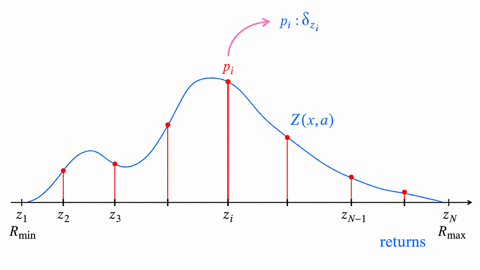
먼저 $[R_{\min},R_{\max}]$ 구간에 $N$개의 $z_i$를 일정한 간격으로 배치한다.

\[\Delta z = \frac{R_{\max}-R_{\min}}{N-1}\] \[z_i = R_{\min}+(i-1)\Delta z, \qquad i=1,\ldots,N\]

따라서 C51이 사용하는 fixed support는 아래와 같이 표현된다.

\[\{z_1,\ldots,z_N\} \subseteq [R_{\min},R_{\max}]\]

Fixed support를 구성하는 각각의 discrete return location $z_i$를 atom이라고 한다. 즉, atom은 C51이 probability mass $p_i(x,a)$를 배정하는 return axis 위의 위치이며, 이 atom들을 모두 모은 집합 ${z_1,\ldots,z_N}$이 support이다.

여기서 $R_{\min}$과 $R_{\max}$는 한 시점의 reward 범위가 아니라, 모델이 표현할 discounted return의 하한과 상한이다.

영역에 표현된 $N$개의 $z_i$는 Dirac delta function $\delta_{z_i}$과 $p_i$라는 확률 질량으로 표현된다.

\[Z_\theta(x,a) = \sum_{i=1}^{N}p_i(x,a)\delta_{z_i}\]

여기서, $\delta_{z_i}$는 Dirac delta function으로,

\(\delta_{z_i}(x) = \begin{cases} \infty, & x = z_i,\\ 0, & x \neq z_i. \end{cases}, \qquad \int_{-\infty}^{\infty} \delta_{z_i}(x)\,dx = 1\) discrete한 상황에서 위치를 표현할때 자주 사용된다.

$p_i(x,a)$는 state $x$에서 action $a$를 선택했을 때 return이 $z_i$에 놓일 probability이며, 다음 조건을 만족한다.

\[p_i(x,a)\ge 0, \qquad \sum_{i=1}^{N}p_i(x,a)=1\]

이렇게 연속확률분포를 fixed support위에 discrete 확률분포로 근사화하면 모델은 확률질량 $p_i(x,a)$를 학습하게 된다.

Softmax를 이용한 Probability Parameterization

Neural network는 각 action에 대해 $N$개의 $\theta_i(x,a)$를 출력하고, 각 probability $p_i(x,a)$는 이 $\theta_i(x,a)$에 softmax를 적용하여 계산한다.

\[p_i(x,a) = \frac{\exp(\theta_i(x,a))} {\sum_{j=1}^{N}\exp(\theta_j(x,a))}, \qquad i=1,\ldots,N\]

따라서 직접 학습되는 것은 서로 독립된 probability $p_i$가 아니라 network parameter $\theta_i$이다.

Discrete action의 개수가 $

\mathcal{A}

$라면 마지막 layer는 action마다 $N$개의 $\theta_i$를 출력하므로, 총 Network output의 dimension은 $ N\lvert\mathcal{A}\rvert $이 된다.

C51이라는 이름과 Support 범위

재밌는건 C51이라는 이름은 fixed support ${z_1,\ldots,z_N}$의 개수 $N=51$여서 붙여진 이름이다.

이때 $R_{\min}$과 $R_{\max}$의 선택이 중요하다. Support 범위를 너무 좁게 설정하면 범위 밖의 return을 표현할 수 없고, 이후 Bellman target을 projection할 때 probability mass가 양 끝의 $z_1, z_N$으로 모이게 된다. 반대로 같은 $N$에서 범위를 너무 넓게 설정하면 $\Delta z$가 커져 return distribution을 세밀하게 표현하기 어렵다. 따라서 예상되는 discounted return의 범위와 필요한 resolution을 함께 고려해 두 경계를 정해야 한다.

Bellman Update

\[(\mathcal{T}Z_{\tilde{\theta}})(x,a) \mathrel{\overset{D}{=}} r+\gamma Z_{\tilde{\theta}}(x',\arg\max_{a'}\mathbb{E}[Z_{\tilde{\theta}}(x',a')] )\]

여기서 bellman target을 만드는 target network parameter는 일정한 업데이트동안 고정되므로, $\theta$가 아닌 $\tilde{\theta}$로 표기한다.

bellman update가 적용된 target distiibution은 기존 $Z_{\tilde{\theta}}(x’,a’)$의 support를 벗어나게 된다. 이떄문에 disjoint support 문제가 발생한다.

disjoint support 문제

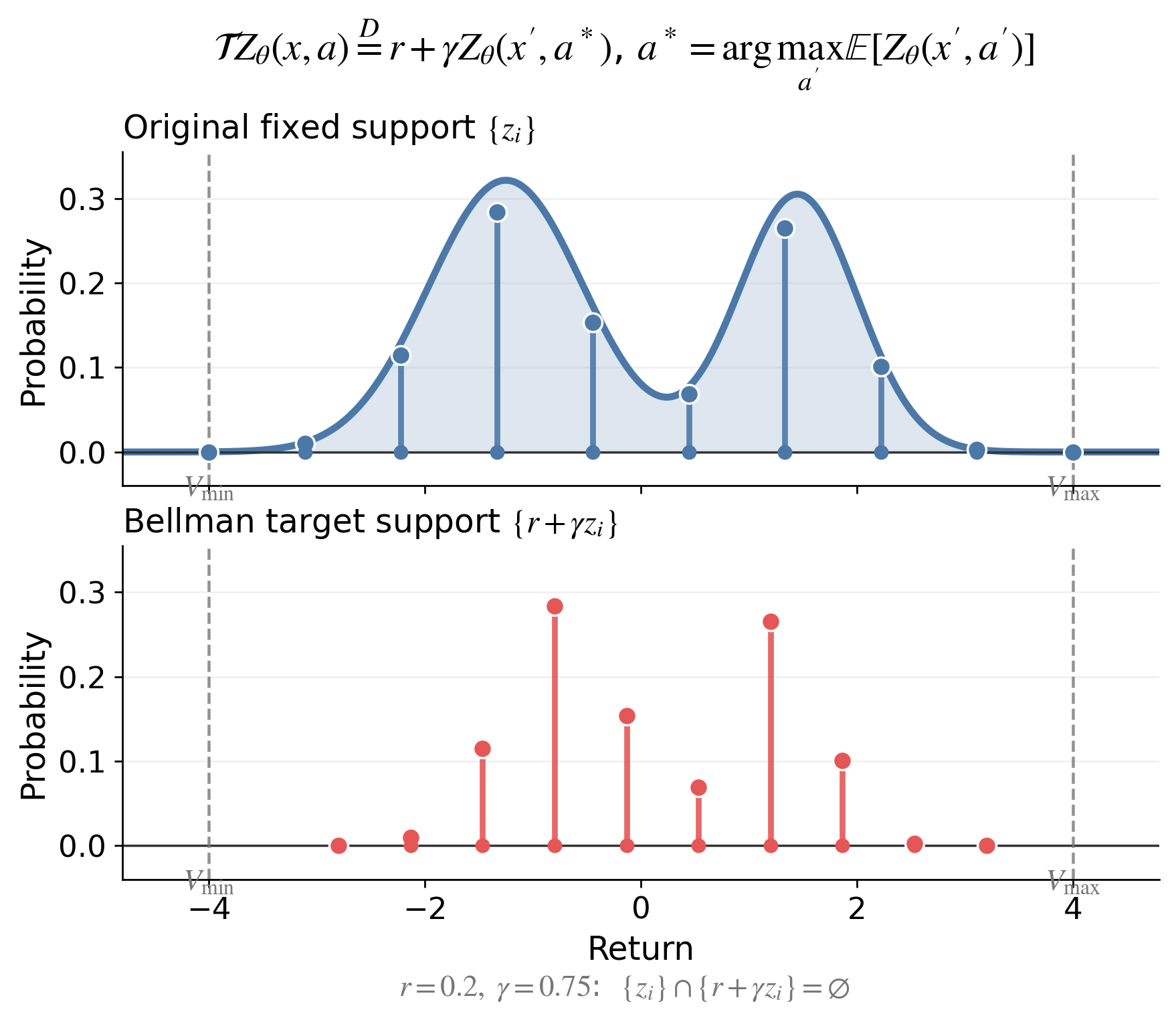
위 이미지가 disjoint support문제를 가장 잘 보여준다. original distribution을 근사한 $Z_\theta(x,a)$는 fixed support ${z_1,\ldots,z_N}$ 위에 있다. 여기서 Bellman update를 적용하면, reward $r$만큼 이동하고 discount factor $\gamma$만큼 간격이 줄어든 새로운 distribution $(\mathcal{T}Z_{\tilde{\theta}})(x,a)$가 만들어진다. 이때 $(\mathcal{T}Z_{\tilde{\theta}})(x,a)$의 support는 원래의 fixed support와 일반적으로 일치하지 않는다.

이러한 disjoint support문제를 해결하기 위해 Wasserstein metric을 보통 사용하지만 실제 학습에서는 해당 metric은 SGD를 적용하기가 어렵고, control의 경우 distributional instability문제가 이 metric을 직접 사용하는 것을 막는다.

Projection

C51은 이러한 문제를 projection을 통해 해결한다. disjoint support 문제는 bellman update가 발생할때마다 support가 이동하면서 발생하는데, 이를 막기 위해 bellman update가 된 distribution을 원래의 fixed support로 projection하여, 항상 같은 support를 가지도록 만든다.

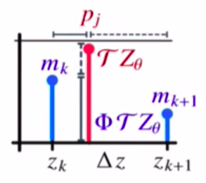
bellman update된 $\hat{z}j$가 fixed support의 이웃한 두 $z_k$와 $z{k+1}$ 사이에 있다고 하자.

\[z_k \le \hat{z}_j \le z_{k+1}\]

Target $\hat{z}j$이 가지고 있던 probability $p{\tilde{\theta},j}(x’,a^*)$는 가까운 fixed $z_i$일수록 더 큰 weight를 받도록 두 이웃에 선형 보간하고 기존 위치에서의 probability mass는 제거한다.

\[m_k \leftarrow m_k + p_{\tilde{\theta},j}(x',a^*) \frac{z_{k+1}-\hat{z}_j}{\Delta z}\] \[m_{k+1} \leftarrow m_{k+1} + p_{\tilde{\theta},j}(x',a^*) \frac{\hat{z}_j-z_k}{\Delta z}\]

두 interpolation weight의 합은 1이므로 기존 probability mass는 보존된다.

KL-Divergence

이 과정을 통해 우리는 disjoint support 문제를 해결하고, update되는 distribution과 기존 distribution사이의 KL divergence를 계산할 수 있다. KL divergence를 최소화하는 방향으로 online network를 update하면, projected bellman target distribution과 online network의 prediction distribution이 가까워지도록 학습할 수 있다.

\[D_{\mathrm{KL}}\left( \Phi\widehat{\mathcal{T}}Z_{\tilde{\theta}}(x,a) \mathbin{\|} Z_\theta(x,a) \right)\]

위 식에서 $\mathcal{T} Projected target probability를 $m_i$, online network의 prediction을 $p_{\theta,i}(x,a)$라고 하면 KL divergence는 다음과 같이 분해된다.

\[D_{\mathrm{KL}}(m\mathbin{\|}p_\theta) = \sum_{i=1}^{N}m_i\log m_i - \sum_{i=1}^{N}m_i\log p_{\theta,i}(x,a)\]

Gradient를 계산하는 동안 $m_i$는 fixed target network $\tilde{\theta}$에서 만든 상수로 취급한다. 따라서 첫 번째 항은 online network parameter $\theta$와 무관하며, KL divergence를 최소화하는 것은 두 번째 항의 음수인 cross-entropy loss를 최소화하는 것과 같다.

\[\mathcal{L}_{x,a}(\theta) = -\sum_{i=1}^{N}m_i\log p_{\theta,i}(x,a)\]

즉, C51은 sample Bellman target을 fixed support 위로 projection한 뒤, projected distribution을 classification target처럼 사용하여 online network를 update한다. Target network $\tilde{\theta}$는 매 gradient step에서 고정되며, 정해진 주기마다 online network $\theta$의 parameter로 갱신된다.

C51의 전체 과정

전체 과정을 순서대로 정리하면 다음과 같다.

1. $(a)$: continuous한 return distribution를 fixed support ${z_1,\ldots,z_N}$ 위의 categorical distribution $Z_{\tilde{\theta}}(x’,a^*)$으로 근사한다.
2. $(b)$: Discount factor $\gamma$를 곱하면 support와 distribution의 폭이 $\gamma$배로 줄어든다.
3. $(c)$: Reward $r$을 더하면 distribution 전체가 $r$만큼 이동하여 Bellman target $\widehat{\mathcal{T}}Z_{\tilde{\theta}}$가 된다.
4. $(d)$: Projection $\Phi$가 각 target $\hat{z}_i$를 fixed support위로 projection시킨다.

이렇게 얻은 $\Phi\widehat{\mathcal{T}}Z_{\tilde{\theta}}$는 $Z_\theta(x,a)$와 동일한 fixed support를 가지므로, C51은 두 categorical distribution을 비교하여 online network를 학습할 수 있다.

DQN에서 C51로 바뀌는 Update Block

C51은 DQN의 environment interaction, $\epsilon$-greedy action selection, replay buffer, target network 구조를 그대로 사용한다. 달라지는 핵심은 아래 이미지에서 핑크 박스안에 있는 replay buffer에서 minibatch를 꺼낸 뒤 network를 update하는 부분이다.

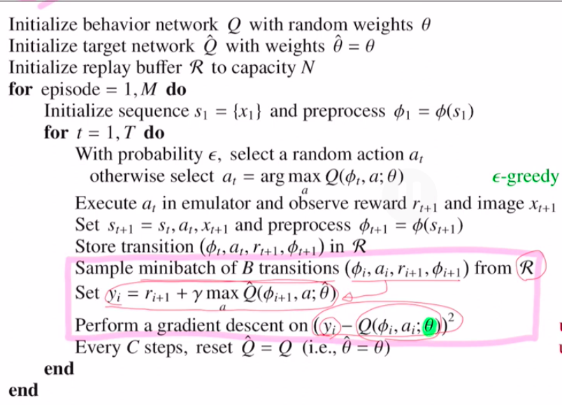
위 DQN algorithm에서 강조된 세 줄은 C51의 projected distribution update와 다음과 같이 대응된다. 아래에서 $\ell$은 minibatch 안의 transition index이고, $i$는 $z$의 index이다.

단계	DQN	C51
Minibatch sampling	Replay buffer에서 transition minibatch를 추출한다.	같은 방식으로 transition minibatch를 추출한다.
Bellman target	Scalar target $y_\ell=r_{\ell+1}+\gamma\max_a Q_{\tilde{\theta}}(x_{\ell+1},a)$를 계산한다.	Categorical Bellman target을 계산하고 fixed support 위로 projection하여 target probabilities $m_{\ell,i}$를 만든다.
Network update	Squared TD error $(y_\ell-Q_\theta(x_\ell,a_\ell))^2$를 최소화한다.	Cross-entropy $-\sum_i m_{\ell,i}\log p_{\theta,i}(x_\ell,a_\ell)$를 최소화한다.

즉, minibatch를 replay buffer에서 sampling하는 구조 자체는 유지된다. 그 뒤 하나의 scalar target과 squared error를 사용하던 두 단계가, $N$개 $z$의 projected target distribution과 cross-entropy를 사용하는 단계로 바뀐다. 나머지 DQN training loop는 거의 그대로 사용할 수 있다.

C51 Projected Bellman Update Algorithm

달라지는 부분을 algorithm으로 정리하면 다음과 같다.

$$ \begin{array}{l} \textbf{Input : } \text{transition }(x_t,a_t,r_{t+1},x_{t+1}),\ \gamma,\ \{z_i\}_{i=1}^{N} \\ \quad Q_{\tilde{\theta}}(x_{t+1},a)\leftarrow\displaystyle\sum_{i=1}^{N}z_i p_{\tilde{\theta},i}(x_{t+1},a) \\ \quad a^*\leftarrow\displaystyle\arg\max_a Q_{\tilde{\theta}}(x_{t+1},a) \\ \quad m_i\leftarrow 0,\quad i=1,\ldots,N \\ \quad \textbf{for }j=1,\ldots,N\ \textbf{do} \\ \quad \quad\quad \hat{z}_j\leftarrow\left[r_{t+1}+\gamma z_j\right]_{R_{\min}}^{R_{\max}} \\ \quad \quad\quad b_j\leftarrow\dfrac{\hat{z}_j-R_{\min}}{\Delta z}+1 \\ \quad \quad\quad k\leftarrow\lfloor b_j\rfloor \\ \quad \quad\quad m_k\leftarrow m_k+p_{\tilde{\theta},j}(x_{t+1},a^*)(k+1-b_j) \\ \quad \quad\quad\quad m_{k+1}\leftarrow m_{k+1}+p_{\tilde{\theta},j}(x_{t+1},a^*)(b_j-k) \\ \quad \textbf{end for} \\ \textbf{return }\mathcal{L}_{x_t,a_t}(\theta)\leftarrow-\displaystyle\sum_{i=1}^{N}m_i\log p_{\theta,i}(x_t,a_t) \end{array} $$

QR-DQN

QR-DQN은 C51과 마찬가지로 return distribution을 $N$개의 Dirac measure로 근사하지만, 무엇을 고정하고 무엇을 학습하는지가 다르다. C51은 return 위치 $z_i$를 고정하고 probability $p_i(x,a)$를 학습한다. 반대로 QR-DQN은 각 $z_i$의 probability를 $1/N$로 고정하고 return location $\theta_i(x,a)$를 학습한다.

Quantile Distribution Parameterization

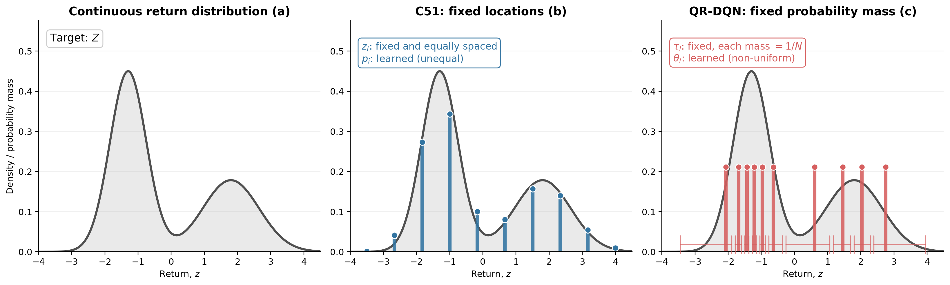
(a) : 근사하려는 continuous return distribution (b) :가운데 C51은 고정된 locations $z_i$마다 서로 다른 probability $p_i$를 학습 (c) QR-DQN은 각 quantile location의 probability를 $1/N$로 고정하고, return locations $\theta_i(x,a)$를 학습

먼저 probability 구간 $[0,1]$을 $N$개의 동일한 크기로 나눈 quantile boundary를 정의한다.

\[\tau_0=0, \qquad \tau_i=\frac{i}{N}, \qquad i=1,\ldots,N\]

각 구간 $[\tau_{i-1},\tau_i]$의 midpoint는 다음과 같이 표현한다.

\[\hat{\tau}_i = \frac{\tau_{i-1}+\tau_i}{2} = \frac{2i-1}{2N}\]

Network output $\theta_i(x,a)$는 true return distribution의 inverse CDF를 quantile midpoint $\hat{\tau}_i$에서 평가한 return location을 근사한다.

\[\theta_i(x,a) \approx F_{Z(x,a)}^{-1}(\hat{\tau}_i)\]

이 locations에 동일한 probability mass $1/N$을 배정하여 quantile distribution을 다음과 같이 모델링한다.

\[Z_\theta(x,a) = \frac{1}{N} \sum_{i=1}^{N} \delta_{\theta_i(x,a)}\]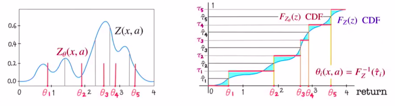

왼쪽 그림에서 파란 곡선은 true return distribution $Z(x,a)$이고, 빨간 세로선은 QR-DQN이 학습하는 return locations $\theta_i(x,a)$이다. 오른쪽에서 하늘색 곡선은 true CDF $F_Z(z)$이고, 빨간 계단은 QR-DQN이 근사한 CDF $F_{Z_\theta}(z)$이다. 각 quantile location에 probability mass $1/N$이 배정되므로 빨간 CDF는 $\theta_i(x,a)$를 지날 때마다 $1/N$만큼 상승한다. 이때 $\theta_i(x,a)$는 true CDF가 $i$번째 구간의 midpoint $\hat{\tau}_i$에 도달하는 return value $F_Z^{-1}(\hat{\tau}_i)$를 근사한다.

모든 $\theta_i$의 probability가 같으므로 scalar action value는 quantile locations의 평균으로 계산한다.

\[\mathbb{E}[Z_\theta(x,a)] = \frac{1}{N}\sum_{i=1}^{N}\theta_i(x,a)\]

QR-DQN이 직접 학습하고 network로 출력하는 대상은 $Q$가 아니라 $Z_\theta$의 quantile locations이다. 위 expectation은 greedy action을 선택할 때만 사용하는 scalar value이며, 별도의 $Q$ output을 학습하는 것이 아니다.

Discrete action의 개수가 $\lvert\mathcal{A}\rvert$라면 network는 action마다 $N$개의 quantile location을 출력하므로, 마지막 layer의 output 개수는 C51과 마찬가지로 $N\lvert\mathcal{A}\rvert$이다. 다만 C51의 output은 probability를 만들기 위한 logits이고, QR-DQN의 output은 return axis 위의 quantile values이다.

구분	C51	QR-DQN
Return locations	$z_i$를 고정	$\theta_i(x,a)$를 학습
Return locations probabilities	Softmax probability $p_i(x,a)$를 학습	$1/N$로 고정
Return 범위	$R_{\min},R_{\max}$를 미리 설정	미리 설정할 필요 없음
Network output	$N\lvert\mathcal{A}\rvert$개의 logits	$N\lvert\mathcal{A}\rvert$개의 quantile values
Bellman target 처리	Fixed support로 projection	별도의 fixed-support projection이 필요 없음

Quantile Regression

QR-DQN은 loss를 Quantile Regression을 이용하여 정의한다. 이를 살펴보기 전에 Quantile Regression이 무엇인지 간단히 알아보자.

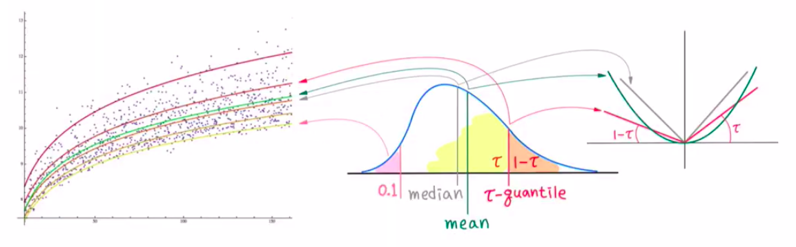
Quantile regression은 L1 regression을 좀더 확장한 regreesion 방법이다. 간단하게 L2 regression -> L1 regression, quantile regression 방법 순으로 설명한다.

L2 regression

Data $x_1,\ldots,x_M$을 하나의 scalar $m$으로 대표하고자 할 때, L2 loss의 minimizer는 sample mean이다.

\[m_{\mathrm{L2}} \in \arg\min_m \sum_{j=1}^{M}(x_j-m)^2\]

실제로 $m$에 대해 미분한 뒤 0으로 두면

\[-2\sum_{j=1}^{M}(x_j-m)=0\]

이므로,

\[m_{\mathrm{L2}} = \frac{1}{M}\sum_{j=1}^{M}x_j\]

를 얻는다.

L1 regression

L1 loss의 minimizer는 sample median이다.

\[m_{\mathrm{L1}} \in \arg\min_m \sum_{j=1}^{M}|x_j-m|\]

Absolute error의 합은 $m$의 왼쪽과 오른쪽에 위치한 sample의 수가 균형을 이룰 때 최소가 되므로 median을 찾는다.

L1 regreesion -> quantile regreesion

Quantile Regression은 이러한 L1 loss를 비대칭적으로 확장한 quantile loss, 또는 pinball loss를 사용한다. $\tau\in(0,1)$에 대한 quantile loss는

\[u=x-q \\ \rho_\tau(u) = \begin{cases} \tau |u|, & u\ge0,\\ (1-\tau)|u|, & u<0 \end{cases}\]

로 정의된다.

즉, prediction $q$가 실제 data $x$보다 작아서 $u>0$인 경우에는 error에 $\tau$를 곱하고, $q$가 $x$보다 커서 $u<0$인 경우에는 error에 $1-\tau$를 곱한다.

주어진 data에서 $\tau$-quantile $q_\tau$는 이러한 quantile loss의 합을 최소화하는 값이다.

\[q_\tau \in \arg\min_q \sum_{j=1}^{M}\rho_\tau(x_j-q)\]

직관적으로 $q_\tau$보다 작거나 같은 데이터가 전체 데이터의 약 $\tau$ 비율을 차지한다. $\tau$가 클수록 $q<x$, 즉 prediction이 data를 underestimate하는 경우에 더 큰 penalty를 부여하므로 높은 quantile을 찾는다. 반대로 $\tau$가 작을수록 낮은 quantile을 찾는다.

특히 $\tau=0.5$이면

\[\rho_{0.5}(u) = \frac{1}{2}|u|\]

이므로 positive constant $1/2$을 제외하면 L1 loss와 같다. 따라서 $0.5$-quantile regression의 minimizer는 median이 된다.

QR-DQN Quantile Regression Loss

앞에서 살펴본 quantile regression을 실제 QR-DQN loss에 적용해 보자. 먼저 next state에서 $Z_{\tilde{\theta}}$의 expectation이 가장 큰 action을 선택한다.

\[a^* \in \arg\max_a \mathbb{E}[Z_{\tilde{\theta}}(x',a)] = \arg\max_a \frac{1}{N} \sum_{j=1}^{N}\tilde{\theta}_j(x',a)\]

선택한 action에 대해 $j$번째 target quantile은 sample Bellman update로 계산한다.

\[\mathcal{T}\tilde{\theta}_j = r+\gamma\tilde{\theta}_j(x',a^*), \qquad j=1,\ldots,N\]

여기서 $\mathcal{T}\tilde{\theta}_j$는 fixed target network로 계산한 target이고, $\theta_i(x,a)$는 현재 behavior, 즉 online network의 prediction이다. Target은 gradient 계산 중 고정하고 $\theta_i(x,a)$만 update한다.

QR-DQN의 Loss function을 quantile regression을 적용하여 다시 써보면 아래와 같다.

\[\mathcal{L}_{\mathrm{QR}}(\theta) = \sum_{i=1}^{N} \mathbb{E}_{J}\left[ \rho_{\hat{\tau}_i} \left( \mathcal{T}\tilde{\theta}_J-\theta_i(x,a) \right) \right] = \frac{1}{N} \sum_{i=1}^{N} \sum_{j=1}^{N} \rho_{\hat{\tau}_i} \left( \mathcal{T}\tilde{\theta}_j-\theta_i(x,a) \right)\]

첫 번째 summation의 $i$는 behavior network의 prediction quantile index이고, 두 번째 summation의 $j$는 target quantile $\mathcal{T}\tilde{\theta}_j$의 index이다. 즉, factor $1/N$은 각 target quantile이 선택될 probability $P(J=j)$에서 나온다.

위 식에서 사용하는 quantile loss는 앞에서 정의한 것과 같다.

\[\rho_\tau(u) = \begin{cases} \tau u, & u\ge 0,\\ (\tau-1)u, & u<0 \end{cases}\]

이 quantile regression loss를 minimize하면 각 $\theta_i$가 midpoint quantile을 학습하며, 그 population minimizer는 다음 절에서 설명할 1-Wasserstein projection의 minimizer와 일치한다. 다만 quantile loss는 $u=0$에서 뾰족하여 미분할 수 없다. 실제 QR-DQN에서는 이를 부드럽게 만들기 위해 Huber loss를 결합한 quantile Huber loss를 사용한다.

\[\mathcal{L}_\kappa(u) = \begin{cases} \dfrac{1}{2}u^2, & |u|\le\kappa,\\ \kappa\left(|u|-\dfrac{1}{2}\kappa\right), & |u|>\kappa \end{cases}\]

Quantile Huber loss는 다음과 같이 정의한다.

\[\rho_\tau^\kappa(u) = \begin{cases} \tau\dfrac{\mathcal{L}_\kappa(u)}{\kappa}, & u\ge 0,\\ (1-\tau)\dfrac{\mathcal{L}_\kappa(u)}{\kappa}, & u<0 \end{cases}\]

$1/\kappa$는 QR-DQN 원 논문의 normalization이며, 흔히 사용하는 $\kappa=1$에서는 첨부한 식과 같은 형태가 된다. $

u

\le\kappa$에서는 quadratic function을 사용하여 0 근처를 smooth하게 만들고, $

u

>\kappa$에서는 linear tail을 유지한다. 실제 loss에서는 위 double summation의 $\rho_{\hat{\tau}i}$를 $\rho{\hat{\tau}_i}^{\kappa}$로 바꾸어 사용한다.

1-Wasserstein Minimization

고정된 state-action pair에서 표기를 간단히 $Z$와 $Z_\theta$로 쓰자. 앞에서 정의한 quantile regression loss와의 관계를 확인하기 위해, true distribution $Z$와 uniform quantile distribution $Z_\theta$ 사이의 1-Wasserstein distance를 inverse CDF로 나타내면 다음과 같다.

\[W_1(Z,Z_\theta) = \sum_{i=1}^{N} \int_{\tau_{i-1}}^{\tau_i} \left| F_Z^{-1}(u)-\theta_i \right|du\]

각 구간의 integral은 $\theta_i$를 해당 구간에 있는 return values의 median으로 둘 때 최소가 된다. 따라서 midpoint quantile

\[\theta_i = F_Z^{-1}(\hat{\tau}_i)\]

를 1-Wasserstein projection의 minimizer로 선택할 수 있다. $F_Z^{-1}$가 $\hat{\tau}i$에서 continuous하다면 이 minimizer는 unique하다. 따라서 각 $\theta_i$가 midpoint quantile을 정확히 추정할수록 $Z\theta$는 $Z$에 대한 1-Wasserstein minimizing approximation에 가까워진다.

즉, QR-DQN은 return bound를 미리 정하거나 Bellman target을 fixed support로 projection하지 않고도, quantile regression을 통해 return locations를 이동시키면서 1-Wasserstein distance를 최소화하는 방향으로 distribution을 학습한다.

C51과 비교한 QR-DQN의 장점

QR-DQN의 장점은 C51과 비교하면 다음과 같이 정리할 수 있다.

1. Preset return bound가 필요하지 않다.

2. Categorical projection이 필요하지 않다. C51은 Bellman target의 atom을 fixed support 위로 projection해야 한다. QR-DQN은 별도의 fixed-support projection을 수행하지 않는다.

3. Wasserstein theory와 실제 objective가 연결된다. C51의 KL divergence는 Wasserstein metric과 직접 연결되지 않는다. 반면 QR-DQN은 quantile regression으로 1-Wasserstein minimizer를 학습하여 이론과 실제 학습의 gap을 줄인다.

다만 이 장점이 nonlinear neural network를 사용하는 control 학습의 global convergence까지 보장한다는 뜻은 아니다. 앞에서 설명한 distributional Bellman optimality operator의 instability는 여전히 별개의 문제이다. QR-DQN이 보장하는 핵심 연결은 quantile regression의 population objective와 1-Wasserstein projection 사이의 일치이다.

QR-DQN Algorithm

$$ \begin{array}{l} \textbf{Input : } \text{transition }(x_t,a_t,r_{t+1},x_{t+1}),\ \gamma,\ N,\ \kappa \\ a^*\leftarrow\displaystyle\arg\max_a\dfrac{1}{N}\sum_{j=1}^{N}\tilde{\theta}_j(x_{t+1},a) \\ \textbf{for }j=1,\ldots,N\ \textbf{do} \\ \quad\quad \mathcal{T}\tilde{\theta}_j\leftarrow r_{t+1}+\gamma\tilde{\theta}_j(x_{t+1},a^*) \\ \textbf{end for} \\ \mathcal{L}_{\mathrm{QR-DQN}}(\theta)\leftarrow\dfrac{1}{N}\displaystyle\sum_{i=1}^{N}\sum_{j=1}^{N} \rho_{\hat{\tau}_i}^{\kappa}\left(\mathcal{T}\tilde{\theta}_j-\theta_i(x_t,a_t)\right) \\ \textbf{return }\mathcal{L}_{\mathrm{QR-DQN}}(\theta) \end{array} $$

QR-DQN도 DQN의 replay buffer, $\epsilon$-greedy exploration, online network와 target network 구조를 유지한다. DQN의 scalar Bellman target과 scalar Huber loss 부분만 $N$개의 target quantile locations와 pairwise quantile Huber loss로 교체한다. C51 algorithm과 달리 target을 fixed support로 projection하는 loop는 없다.

IQN

QR-DQN에서 IQN으로

QR-DQN의 approximation error는 fixed quantile의 개수 $N$에 영향을 받는다. 반면 IQN(Implicit Quantile Network)은 매 update마다 random quantile level $\tau$를 sampling하므로, 고정된 quantile 개수에 제한되지 않고 network capacity와 training 양에 따라 quantile function을 더 정밀하게 근사할 수 있다. 또한 IQN은 학습과 action selection에서 서로 다른 quantile samples $N$, $N’$, $K$를 사용한다. 이를 이해하기 위해 IQN의 quantile sampling 방식과 risk-sensitive policy를 먼저 살펴본다.

Quantile Sampling과 Implicit Distribution

IQN의 network는 state와 action뿐만 아니라 quantile level $\tau$도 입력으로 받는다. 매번 새로 뽑은 base sample $\tau$와 network를 결합하여 return distribution을 정의한다.

\[\tau\sim U([0,1]), \qquad Z_\theta(x,a;\tau) \approx F^{-1}_{Z(x,a)}(\tau)\]

따라서 IQN은 미리 정해진 유한한 atom이나 quantile location 목록을 저장하는 대신, quantile function을 근사하는 network와 base distribution $U([0,1])$를 함께 사용하여 implicit return distribution을 만든다. 이 때문에 IQN을 implicit distributional RL 방법이라고 부른다.

Risk-Sensitive RL

Return distribution을 학습하면 action을 평균 return만으로 비교하지 않고, distribution의 위험도나 특정 tail을 고려하여 선택할 수 있다. 다음 criterion은 이러한 risk-sensitive action selection의 직관을 보여주는 단순한 예시이다.

\[a^*=\arg\max_{a_i}\left( \mathbb{E}[Z(x,a_i)] -\lambda\operatorname{Std}(Z(x,a_i)) \right)\]

$\lambda>0$이면 return의 표준편차가 작은 action을 선호하므로 risk-averse policy가 되고, $\lambda<0$이면 표준편차가 큰 action을 선호하므로 risk-seeking policy가 된다. 이 식에서 $Z(x,a_i)$를 사용하는 이유는 보상 하나가 아니라 해당 action의 return distribution 전체를 고려하기 위해서이다. 이 criterion은 risk-sensitive 선택의 직관을 설명하기 위한 단순한 mean-standard deviation criterion이며, IQN의 고유한 학습 loss를 뜻하지 않는다.

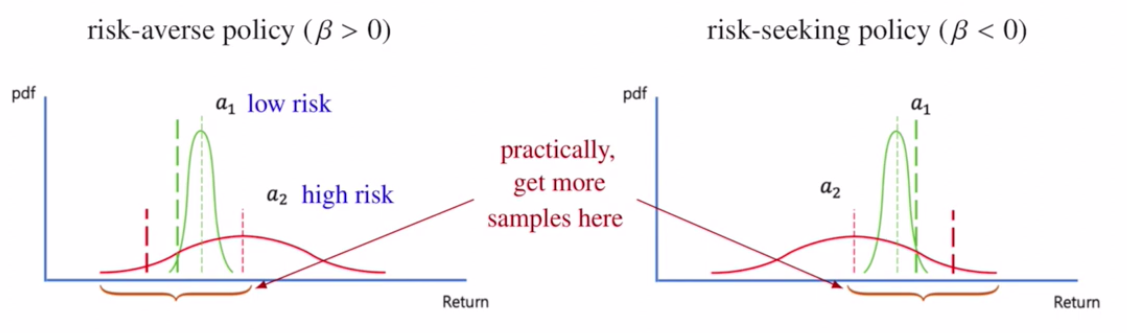
그림의 세로축은 density이므로 곡선의 가장 높은 지점은 mode를 나타낸다. 이는 action의 expected return이나 action selection의 argmax 지점과는 다르다. 왼쪽의 $a_1$은 폭이 좁은 low-risk distribution이고, $a_2$는 폭이 넓은 high-risk distribution이다. $a_2$는 더 높은 return을 얻을 가능성도 있지만, $a_1$보다 낮은 tail return을 얻을 가능성도 함께 가진다. 안정성을 중요하게 생각하는 경우에는 이런 낮은 tail risk 때문에 $a_1$을 선택할 수 있다.

오른쪽은 반대의 직관을 보여준다. 높은 return이 중요한 task라면 high-risk action의 upper tail을 선호할 수 있고, 이때 risk-seeking policy가 high-risk distribution을 선택할 수 있다. 즉 같은 expected return을 사용하는 경우에도 return distribution의 어느 부분을 중요하게 보느냐에 따라 policy가 달라질 수 있다.

여기서 $\lambda$와 뒤에서 정의할 distortion function $\beta$는 서로 다른 개념이다. $\lambda$는 mean-standard deviation criterion에서 risk preference를 표현하는 보조적인 계수이고, $\beta$는 IQN이 quantile level을 변형하여 action value를 계산하는 함수이다.

IQN의 Risk Distortion

IQN은 return distribution 자체를 다시 학습하지 않고도, quantile level에 서로 다른 weight를 주어 risk-sensitive policy를 만들 수 있다. risk-neutral policy에서는 base sample을 그대로 사용한다.

\[\tau\sim U([0,1]), \qquad \beta(\tau)=\tau\]

일반적으로 distortion function $\beta:[0,1]\to[0,1]$를 사용하면 policy가 평가하는 action value를 다음과 같이 정의할 수 있다.

\[Q_\beta(x,a) = \mathbb{E}_{\tau\sim U([0,1])} \left[Z_{\beta(\tau)}(x,a)\right]\]

그리고 action은 다음과 같이 선택한다.

\[\pi_\beta(x)=\arg\max_a Q_\beta(x,a)\]

중요한 점은 risk distortion이 IQN이 학습한 underlying return distribution $Z_\theta$를 바꾸는 것이 아니라, action selection에서 어떤 quantile을 더 중요하게 평가할지를 바꾼다는 것이다. 즉 network가 근사한 quantile function은 그대로 두고, uniform base sample $\tau$에 $\beta$를 적용하여 quantile level의 sampling 또는 weighting만 바꾼다. 따라서 같은 learned distribution에서도 서로 다른 distortion function을 사용하면 서로 다른 risk-sensitive policy를 만들 수 있다.

아래 그림은 모두 세 개의 panel로 구성된다. 왼쪽은 원래 return distribution인 $\mathcal{N}(0,1)$, 가운데는 distortion function $\beta(\tau)$와 risk-neutral 기준인 identity $\beta(\tau)=\tau$의 비교, 오른쪽은 distortion을 적용해 얻은 return samples를 나타낸다. 가운데 panel에서 identity 대각선보다 위에 있는 구간은 원래보다 큰 quantile level을, 아래에 있는 구간은 작은 quantile level을 sampling한다는 뜻이다.

Cumulative Probability Weighting (CPW)

Cumulative Probability Weighting(CPW)은 quantile level의 누적확률을 비선형적으로 변형하는 parameterization이다.

\[\operatorname{CPW}(\eta,\tau) = \frac{\tau^\eta} {\left(\tau^\eta+(1-\tau)^\eta\right)^{1/\eta}}\]

IQN 논문에서 사용한 예시는 $\eta=0.71$이다. CPW는 전체 구간에서 globally convex이거나 globally concave인 함수가 아니다. 작은 $\tau$와 큰 $\tau$에서 curvature가 바뀌므로, CPW를 risk-averse 또는 risk-seeking 중 한쪽 policy로 단순하게 분류할 수 없다. 그림의 가운데 panel에서는 identity와의 차이가 양쪽 끝 구간에서 나타나고, 그 결과 두 tail의 상대적 영향이 함께 조정되는 형태를 확인할 수 있다.

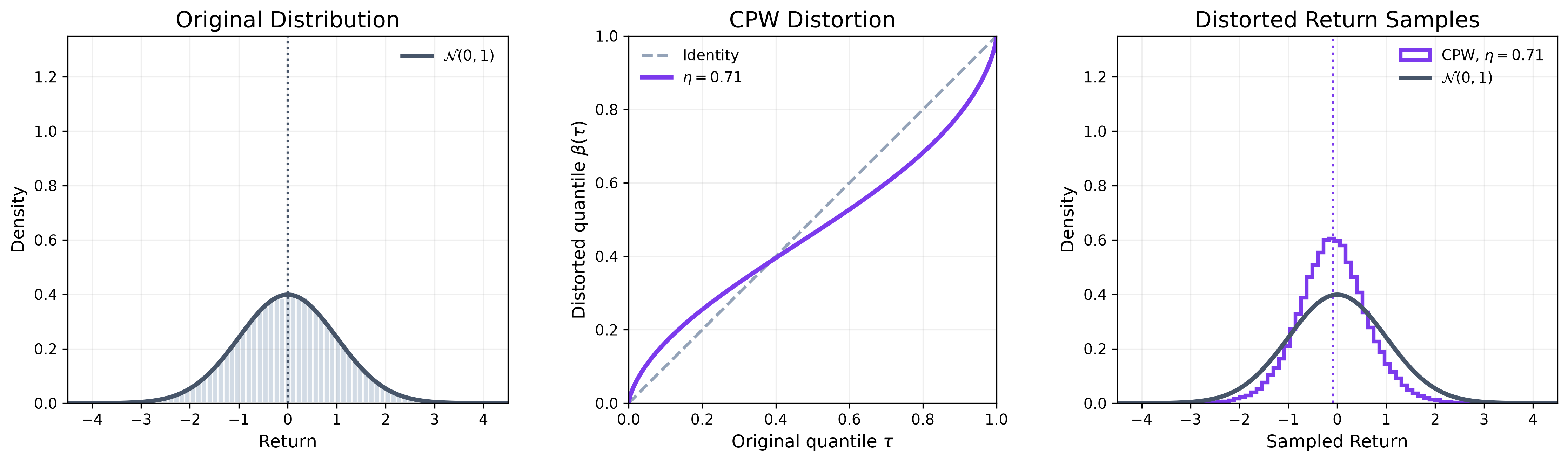
왼쪽의 원래 분포에서 uniform하게 quantile level을 뽑는 대신, 가운데의 CPW curve를 통해 level을 변환하면 오른쪽처럼 sampling된 return distribution이 달라진다. 이 예시는 한쪽 tail만 선택하는 정책이라기보다, lower-tail과 upper-tail을 모두 포함한 quantile weighting의 변화를 보여준다.

Wang Distortion

Wang distortion은 standard Normal distribution의 CDF를 이용하여 quantile level을 이동시킨다.

\[\operatorname{Wang}(\eta,\tau) = \Phi\left(\Phi^{-1}(\tau)+\eta\right)\]

여기서 $\Phi$는 standard Normal cumulative distribution function(CDF)이고, $\Phi^{-1}$는 그 inverse CDF, 즉 quantile function이다. $\eta<0$이면 변환된 level이 lower quantile 방향으로 이동하여 lower return을 더 중요하게 보는 risk-averse policy가 된다. 반대로 $\eta>0$이면 upper quantile 방향으로 이동하여 높은 return을 선호하는 risk-seeking policy가 된다.

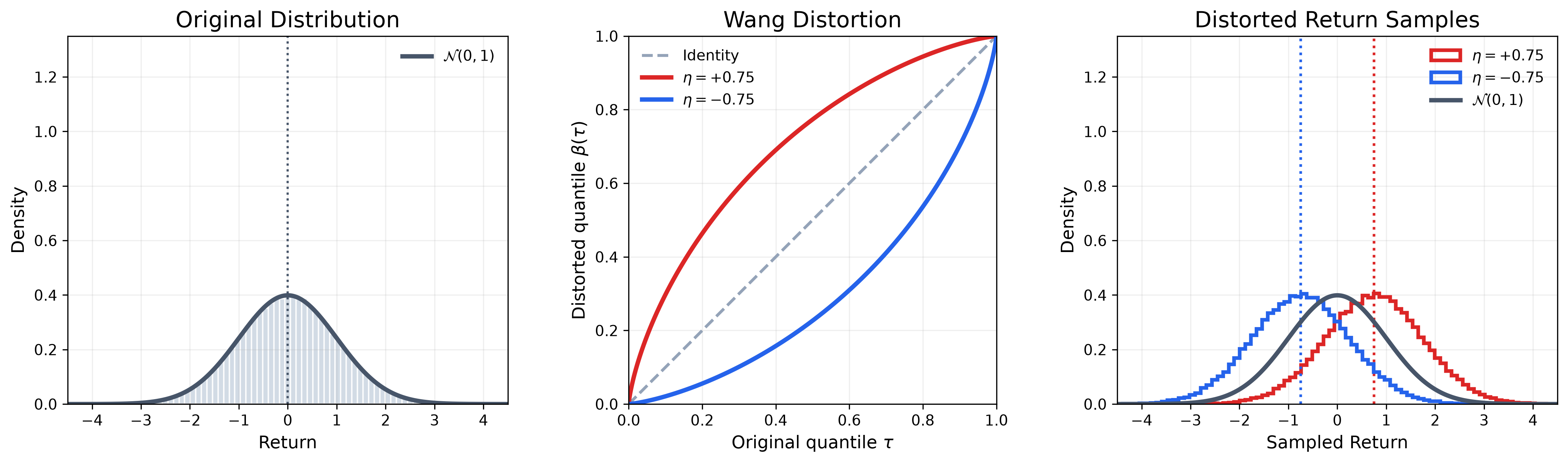
그림에서는 $\eta=+0.75$인 red curve가 upper quantile 방향으로 이동하고, 오른쪽 panel의 red samples도 더 높은 return 쪽으로 이동한다. $\eta=-0.75$인 blue curve는 반대로 lower quantile 방향으로 이동하며, blue samples는 더 낮은 return 쪽에 집중된다.

Power Distortion

Power distortion은 $\eta$의 부호에 따라 lower-tail 또는 upper-tail 방향으로 quantile level을 변환한다.

\[\operatorname{Pow}(\eta,\tau) = \begin{cases} \tau^{\frac{1}{1+|\eta|}}, & \eta\ge 0,\\ 1-(1-\tau)^{\frac{1}{1+|\eta|}}, & \eta<0 \end{cases}\]

$\eta=0$이면 $\operatorname{Pow}(0,\tau)=\tau$가 되어 identity distortion과 같다. $\eta<0$이면 lower quantile 방향으로 변환되어 risk-averse policy가 되고, $\eta>0$이면 upper quantile 방향으로 변환되어 risk-seeking policy가 된다. Wang distortion과 마찬가지로 부호가 어느 tail을 강조할지를 결정하지만, quantile curve의 구체적인 형태는 다르다.

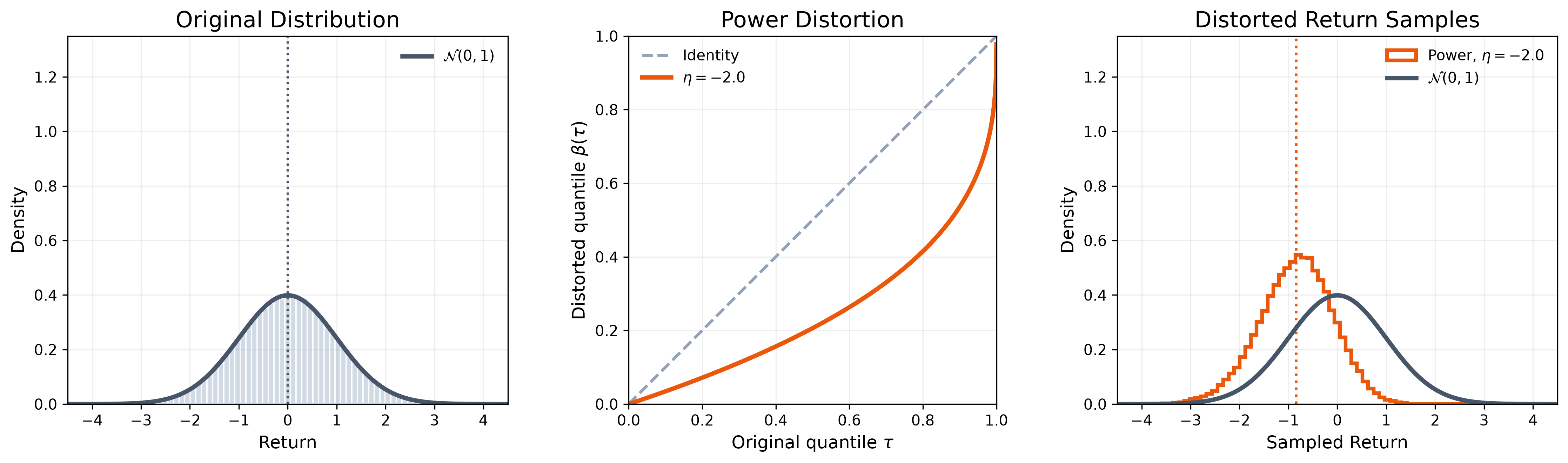
이 그림은 $\eta=-2.0$인 risk-averse example이다. 가운데의 orange curve가 identity보다 lower quantile 방향으로 변환되기 때문에, 오른쪽의 orange return samples가 원래 $\mathcal{N}(0,1)$보다 낮은 return 영역에 집중된다.

Conditional Value-at-Risk (CVaR)

CVaR distortion은 lower-tail의 일정한 비율만 사용하도록 quantile level을 축소한다.

\[\operatorname{CVaR}(\eta,\tau)=\eta\tau, \qquad 0<\eta\le 1\]

$\tau\sim U([0,1])$이면 $\eta\tau\sim U([0,\eta])$이므로, 전체 quantile 중 가장 낮은 $\eta$ 비율만을 sampling하게 된다. 따라서 reward 기준으로는 lower-tail risk를 중시하는 risk-averse policy가 된다. $\eta=1$이면 모든 quantile level을 그대로 사용하므로 identity distortion으로 돌아간다. 이 parameterization은 lower-tail만을 선택하는 formulation이므로 risk-averse policy에만 사용되며, risk-seeking policy를 표현하는 용도는 아니다.

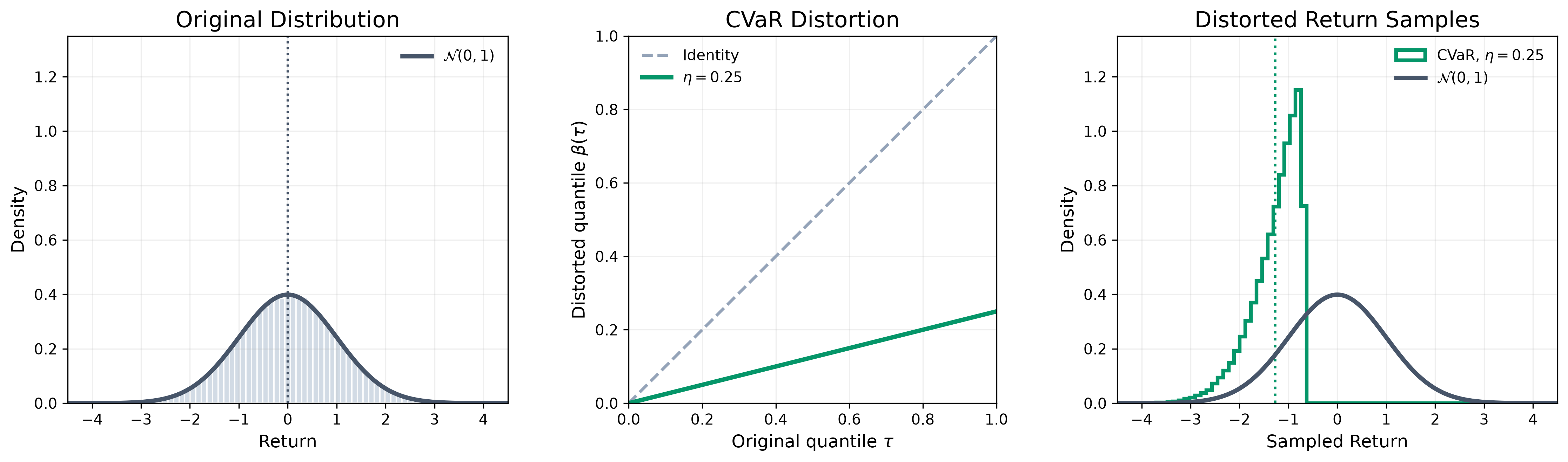
그림의 $\eta=0.25$인 green curve는 $\tau$를 $[0,0.25]$ 구간으로 압축한다. 그 결과 오른쪽 panel의 green samples는 원래 분포의 lower 25% quantile에 해당하는 낮은 return 영역에 집중한다. 즉 평균 return 전체가 아니라 최악의 일부 결과를 기준으로 action을 비교하는 직관을 제공한다.

Algorithm

IQN은 action selection에 사용할 quantile samples와 loss 계산에 사용할 samples를 나누어 다음과 같이 update한다.

$$ \begin{array}{l} \textbf{Input : } \text{transition }(x_t,a_t,r_{t+1},x_{t+1}),\ \gamma,\ N,\ N',\ K,\ \kappa,\ \beta \\ \textbf{for }k=1,\ldots,K\ \textbf{do} \\ \quad\quad \widetilde{\tau}_k\sim\beta(\cdot) \\ \textbf{end for} \\ a^*\leftarrow\arg\max_a\ \dfrac{1}{K}\sum_{k=1}^{K} Z_{\widetilde{\tau}_k}(x_{t+1},a) \\ \textbf{for }i=1,\ldots,N\ \textbf{do} \\ \quad\quad \tau_i\overset{\mathrm{i.i.d.}}{\sim}U([0,1]) \\ \textbf{end for} \\ \textbf{for }j=1,\ldots,N'\ \textbf{do} \\ \quad\quad \tau'_j\overset{\mathrm{i.i.d.}}{\sim}U([0,1]) \\ \textbf{end for} \\ \textbf{for }i=1,\ldots,N\ \textbf{do} \\ \quad\quad \textbf{for }j=1,\ldots,N'\ \textbf{do} \\ \quad\quad\quad\quad \delta_{ij}\leftarrow r_{t+1}+\gamma\widetilde{Z}_{\tau'_j}(x_{t+1},a^*) \\ \quad\quad\quad\quad\quad\quad\quad\quad\ -Z_{\tau_i}(x_t,a_t) \\ \quad\quad \textbf{end for} \\ \textbf{end for} \\ \mathcal{L}\leftarrow\dfrac{1}{N'}\sum_{i=1}^{N}\sum_{j=1}^{N'}\rho_{\tau_i}^{\kappa}(\delta_{ij}) \\ \textbf{return }\mathcal{L} \end{array} $$

알고리즘에서 $K$는 action selection에 사용하는 sample 수이다. risk-sensitive policy에서는 $\widetilde{\tau}_k\sim\beta(\cdot)$로 distorted samples를 사용하고, risk-neutral policy에서는 $\beta(\tau)=\tau$이므로 uniform samples를 사용한다.

$N$은 online prediction network의 quantile samples, $N’$은 target network의 quantile samples이다. 두 sample 모두 loss 계산에 사용되므로 $\tau_i$와 $\tau’_j$는 uniform distribution에서 뽑는다.

따라서 distortion $\beta$는 action을 선택하는 $K$ samples에만 적용되고, loss를 계산하는 $\tau_i$, $\tau’_j$에는 적용되지 않는다. $N$, $N’$, $K$는 서로 다른 역할을 가지므로 각각 별도로 조절할 수 있다.

Network Structure

IQN은 DQN의 state representation에 quantile level을 위한 embedding branch를 추가한다. DQN의 convolutional layers가 state $x$를 feature vector로 바꾸는 함수를 $\psi$라고 하면

\[\psi:\mathcal X\to\mathbb R^d, \qquad Q(x,a)\approx f(\psi(x))_a\]

로 나타낼 수 있다. 여기서 $\psi(x)$는 CNN이 state에서 계산한 state feature vector이고, $f(\psi(x))_a$는 action $a$의 scalar value이다. IQN은 quantile level $\tau$를 $d$차원 feature로 바꾸는 함수 $\phi$를 추가한다.

\[\phi:[0,1]\to\mathbb R^d\]

논문에서는 cosine basis와 fully-connected layer, ReLU를 사용하여 quantile embedding을 계산한다.

\[\phi_j(\tau) = \operatorname{ReLU}\left( \sum_{i=0}^{n-1}\cos(\pi i\tau)w_{ij}+b_j \right), \quad j=1,\ldots,d, \quad n=64\]

$w_{ij}$와 $b_j$는 학습되는 embedding parameters이며, $n=64$는 cosine basis component의 개수이다. State feature와 quantile feature는 기본적으로 element-wise Hadamard product로 결합한다.

\[Z_\tau(x,a) \approx f\left(\psi(x)\odot\phi(\tau)\right)_a\]

아래 구조에서 위쪽 경로는 $x\to\mathrm{CNN}\to\psi(x)$를, 아래쪽 경로는 $\tau\to$ cosine embedding $\to\mathrm{FC+ReLU}\to\phi(\tau)$를 나타낸다. 두 feature의 product가 다시 $\mathrm{FC+ReLU}$를 통과하면 각 action에 대한 $Z_\tau(x,a)$가 출력된다.

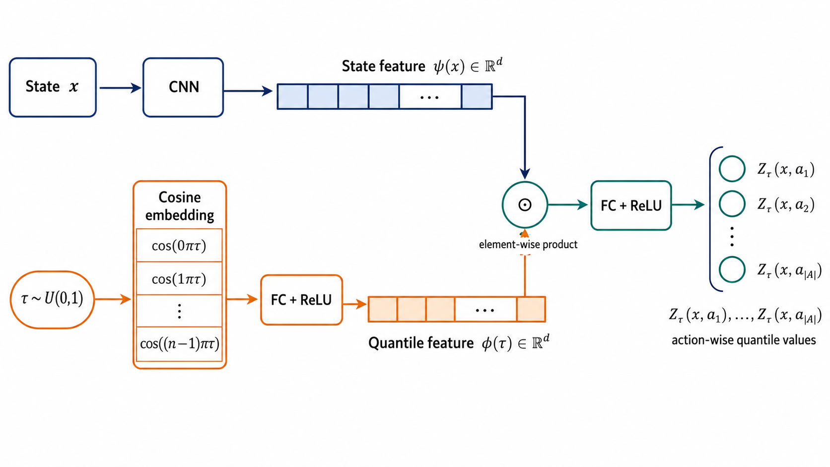
곱셈 결합에는 feature를 이어 붙이는 concatenation 형태와 residual-like한 형태도 사용할 수 있다.

\[f\left([\psi(x)\mathbin\Vert\phi(\tau)]\right)_a\] \[f\left(\psi(x)\odot(1+\phi(\tau))\right)_a\]

이 식들은 update마다 선택하는 연산이 아니라 network architecture의 대안이며, 본문 그림과 기본 구현에서는 multiplicative form인 $\psi(x)\odot\phi(\tau)$를 사용한다.